Pulsar Analysis Tutorial

This tutorial illustrates the flow of a basic pulsar analysis, using the following pulsar tools:

Pulsar Tools:	Tool Tutorials:
gtpsearch	Period Search Tutorial
gtpspec	Pulsation Search Tutorial
gtptest	Periodicity Test Tutorial
gtpphase	Pulse Phase Calculation
gtophase	Binary Orbital Phase Calculation
gtephem	Ephemeris Computation Utility
gtpulsardb	Ephemeris Data File
gtbary	Arrival Time Correction
Also see: Overview: Pulsar Analysis

Notes:

• The tutorials for each tool are available from the 2nd-level, Pulsar Analysis navbar that can be accessed from:

  bluenavbar --> Pulsar Analysis

• The Science Tools References for each of these tools are available from the 3rd-level navigation bar which can be accessed from:

  bluenavbar --> SciTools References -- Pulsar (Tools)

To launch the popup window for the 2nd-level "Pulsar Analysis" navigation bar, click on: Pulsar Analysis Tutorials

Tip: You can also launch this popup by clicking on the blue Timing Analysis button on the left side of the Pulsar Analysis navigation bar, but only when it is displayed in its normal 2nd-level position (i.e., not when it is displayed in a popup). If you wish, you also display a second popup window for the Science Tools References. (This popup is also linked to the Open in New Window button on the 2nd-level SciTools References navigation bar.)

Prerequisites

• event data file in FT1 format 
  (sometimes referred to as the photon data file)

• spacecraft data file in FT2 format
  (also referred to as the pointing and livetime history file)

• fhisto (FTOOLS) available from the: Goddard Space Flight Center (GSFC) website

Note: Required in step 5; not provided with Science Tools distribution.
(You may also want to download: fplot, fv, and fdump.)

Links:

• Appendix A. Binary Modulation and Orbital Phase

• Appendix B. Notes on Numerical Computation

• Appendix C. Temporal Analysis with Non-GLAST Analysis Tools

Steps

1. Extract and Select the Data

2. Familiarize Yourself with Ephemeris Information

3. Calculate Pulse Phase for Each Photon

4. Use Pulse Phases in Your Analysis

1. Extract and Select the Data

Download data, screen events as you do for your spectral or image analysis.

See:

• Extract LAT Data

• Explore LAT Data: Map and Lightcurve

Note: For maximum pulse-detection sensitivity, select only events within a relatively small spatial region, typically of size of a couple of PSF's; steady flux is a "noise" for your periodicity searches and for periodicity significance tests.

2. Familiarize Yourself with Ephemeris Information

Two sets of parameters are commonly used in pulsar timing analyses:

• spin parameters, that characterize pulsar's spin frequency, and

• orbital parameters, that characterize a pulsar's orbit around its companion star if it is in a binary system

These parameters (the ephemeris information of your pulsar) may or may not be available for your analysis; if they are, it will be helpful to collect such information before going any further. You might also find ephemeris information of your pulsar in the pulsar ephemerides database. It is a FITS file containing spin and orbital parameters and other related information for your convenience. If your pulsar is not listed in the database, you might want to look for ephemeris information in the literature. Parameters you need to collect for the pulsar tools include:

• Spin parameters

t0:		an ephemeris epoch, or an arbitrary chosen origin of time
φ0:		pulse phase at time t0
f0:		pulse frequency at time t0
f1:		the 1st time derivative of frequency at time t0
f2:		the 2nd time derivative of frequency at time t0

NOTE: f0, f1, and f2 can be replaced by p0, p1, and p2, which are pulse period at time t0, the 1st time derivative of period at time t0, the 2nd time derivative of period at time t0, respectively.

• Orbital parameters (for binary pulsars only)

PB:		orbital period
PBDOT:		first time derivative of PB (orbital period)
A1:		projected semi-major axis in light seconds
XDOT:		first time derivative of A1 (projected semi-major axis)
ECC:		orbital eccentricity
ECCDOT:		first time derivative of ECC (eccentricity)
OM:		longitude of periastron
OMDOT:		first time derivative of periastron longitude
T0:		barycentric time (TDB scale) of periastron in MJD
GAMMA:		time-dilation and gravitational redshift parameter
SHAPIRO_R:		range parameter of Shapiro delay in binary system
SHAPIRO_S:		shape parameter of Shapiro delay in binary system

Special Settings for L&EO 55-day Simulation Data

The pulsar ephemerides database for L&EO 55-day Simulation Data is available at the GSSC data server together with the simulated photon data. If you plan to use the database file in your analysis with our pulsar analysis tools, run the following commands once prior to your pulsar analysis. This will modify your parameter files for the pulsar analysis tools, so that you don't have to type the name of solar system ephemeris everytime you run those tools.

ShellPrompt: pset gtbary solareph="JPL DE200"
ShellPrompt: pset gtephem solareph="JPL DE200"
ShellPrompt: pset gtophase solareph="JPL DE200"
ShellPrompt: pset gtpphase solareph="JPL DE200"
ShellPrompt: pset gtpsearch solareph="JPL DE200"
ShellPrompt: pset gtpspec solareph="JPL DE200"
ShellPrompt: pset gtpulsardb solareph="JPL DE200"

Another note on this particular database file is a special naming convernsion used for pulsar names in the database file. The names in the database file are based on a conventional PSR B/J-name, except that 1) a white space after "PSR" is replaced with an underscore ("_"), and 2) a plus sign ("+") and a minus sign ("-") are replaced with a character "p" and "m", respectively. For example, the Crab pulsar, a.k.a., "PSR B0531+21", is "PSR_B0531p21" in the database file, and the Vela pulsar, a.k.a., "PSR B0833-45", is "PSR_B0833m45" in the database file. You can list all the pulsar names listed in the database file by running the following command.

ShellPrompt: fdump page=no prhead=no
Name of FITS file and [ext#][] data/pulsardb_LEO55.fits[1]
Name of optional output file[STDOUT] STDOUT
Names of columns[] PSRNAME
Lists of rows[-] -
 
 
        PSRNAME
 
      1 PSR_B0833m45
      2 PSR_B0531p21
      3 PSR_J0633p1746
      4 PSR_B1706m44
      5 PSR_B1055m52
      ...

Our pulsar analysis tools understand only names listed in a database file that is given to them. In your analysis with the pulsar ephemerides database for L&EO 55-day Simulation Data, give the name of your pulsar in the above format to the pulsar tools, so that the tools can find appropriate ephemerides for you.

3. Calculate Pulse Phase for Each Photon

Sample Files. To try the examples in this section, you can download the following fake data files:

• my_pulsar_events_v3.fits (1.9 MB)

• my_pulsar_spacecraft_data_v3r1.fits (108 kB)

• master_pulsardb_v3.fits (248 kB).

Note: Both of these examples will result in an identical event file and, in both cases, the event file processed by gtpphase will be identical to:

• my_pulsar_events_phase_v3.fits (1.9 MB)

which is also available for download for your comparison.

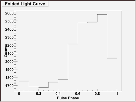
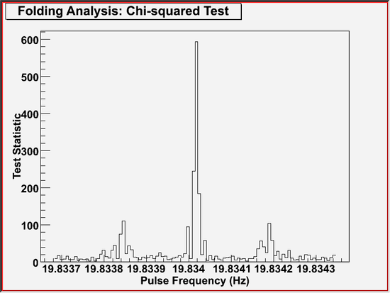
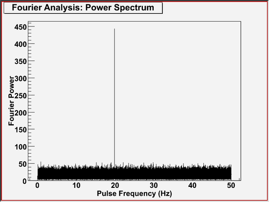
With ephemeris information of your pulsar, you can test periodicity in your dataset, and calculate a pulse phase for each photon in your dataset. Below are a few example cases in assigning pulse phases to photons in your dataset.

Case 1: Using Exact Ephemerides in the Pulsar Ephemerides Database

The pulsar ephemeris database may contain all ephemeris information necessary for your pulsar analysis. In that case, you might want to simply assume those ephemerides are good enough for your analysis and use them as is. In order to do that, however, the entire dataset must be covered by one or more ephemerides for your pulsar, because each ephemeris in the pulsar ephemerides database has a validity time window, during which the ephemeris data is supposed to be reliable.

To see if the entire dataset of yours is covered by valid ephemerides for your pulsar, you can run gtpphase to compute pulse phases for all photons in your dataset and write them back to your event file. For each photon, gtpphase picks an ephemeris from the database, whose validity time windows covers the photon arrival time. If it finds a photon without a valid ephemeris for it, it produces an error message. In that case, you fall in the other cases described below.

In the following example, gtpphase processes the event file named my_pulsar_events_v3.fits using an pulsar ephemeris (or ephemerides) in the pulsar ephemerides database named master_pulsardb_v3.fits for the pulsar named "PSR B0540-69." gtpphase modifies the event file (my_pulsar_events_v3.fits) in place and nothing will be displayed when the input file is successfully processed.

You can use gtptest to run several periodicity tests to check ephemeris information in the database is good for your dataset. It reads pulse phases that have just been assigned by gtpphase, performs statistical tests for periodicity on them, and displays the test results.

When successful, gtptest produces a test output and a graphical plot of a folded light curve on your screen. In this particular example, the following outputs will be displayed, showing a strong pulsation in the data.

Case 2: Refining Ephemerides in the Pulsar Ephemerides Database

Even if the entire database is not covered by the pulsar ephemerides database, you can still use it for your analysis by refining pulsar ephemerides in the database for your particular dataset. The first step of your analysis in this case is to find an ephemeris entry for your pulsar in the database.

You can run gtephem to check if your pulsar is listed in the pulsar ephemerides database. In the following example, gtephem searches for a pulsar by name and by observation time, computes estimated ephemeris of your pulsar at the observation time, and displays the result of computation. If it cannot find any ephemeris for your pulsar, it will produce a message stating it could not find any. In that case, you may need to try Case 3 or Case 4 described below.

With the successful result above, now you know at least one ephemeris is found in your database that can be used for your analysis. To find out how precise this ephemeris is at the time of your observation, you can run gtpsearch using the same pulsar ephemerides database.

In the following example, gtpsearch reads the event file named my_pulsar_events_v3.fits and performs periodicity tests called "chi-squared test" with 10 phase bins. Periodicity tests are performed at 100 trial pulse frequencies, which are automatically determined such that they are separated from each other by half a Fourier resolution, and that they center at the expected pulse frequency at the time origin of periodicity test, where the expected pulse frequency is determined by an pulsar ephemeris (or ephemerides) in the pulsar ephemerides database named master_pulsardb_v3.fits for the pulsar named "PSR B0540-69". As shown below, gtpsearch pops up a window showing a plot of test statistics as a function of frequency.

In this particular example, the maximum value of the chi-squared test statistic (a.k.a., S-value in the literature) appears at the exact center of the frequency range, because the ephemeris in the database is precise enough at the time of this observation. In general cases, though, the peak may show up in a different place in the plot.

Once you know the pulse frequency at the time of observation, you can use it as if it were taken from the literature in the following analysis, if you would like to. In that case, you may choose to assume all frequency derivatives to be negligible and set them to zero, or you may want to to determine frequency derivatives by yourself. For the former, continue on Case 3, and follow the description there with setting frequency derivatives to zeros. The latter case is beyond the scope of this tutorial and not described here.

Case 3: Using Pulsar Ephemeris in the Literature

You can run gtpsearch with specifying pulsar's spin parameters (pulse frequency or pulse period, and its time derivatives) by numbers, that are taken from the literature, for example.

In the following example, gtpsearch does the same thing as above, using 19.83401688366839422996, -1.8869945816704768775044e-10, and 0.0 for the pulse frequency and its first and second derivatives at the ephemeris epoch of 54368.11094817 MJD (TDB), respectively.

You can also run gtpphase with the same pulsar's spin parameters as above.

In the following example, gtpphase does the same thing as above, using 19.83401688366839422996, -1.8869945816704768775044e-10, and 0.0, for the pulse frequency, its first and second time derivatives at the ephemeris epoch of 54368.11094817 MJD (TDB), respectively.

Case 4: Determining Pulsar Ephemeris Yourself

If your pulsar is not listed in the database nor in the literature, you might want to determine ephemeris on your own by analyzing your data. One way to do it is to run gtpspec. In the following example, gtpspec reads the event file named my_pulsar_events_v3.fits and performs Discrete Fast Fourier Transform (DFFT) with 10~ms time bins. The entire data set is broken up into data segments of 1,000,000 time bins (i.e., 100 ks in length), for each of which A DFFT will be performed and its Fourier power will be computed. Then, the Fourier powers of all the segments are summed up. The pulsar name "PSR B0540-69" is used to look up for a binary orbital parameter in the pulsar ephemerides database named master_pulsardb_v3.fits.

Frequency derivatives may be determined by running this tool multiple times with different combinations of frequency derivatives (given to the tool as ratios over frequency). Use caution when interpreting chance probability, because the tool can only compute it for the number of degrees for each run, not a set of runs with various frequency derivatives. You have to compute a correct chance probability for such analysis, based on the information displayed on the screen such as the number of independent trials for each run. The details on a full pulsation search are beyond the scope of this tutorial and not described here.

Once you determine the pulse frequency at the time of observation, you can use it in Case 3 as if it were taken from the literature in the following analysis.

4. Use Pulse Phases in Your Analysis

Sample File. To try the examples in this section, you can download the following fake data file:

• my_pulsar_events_phase_v3.fits (1.9 MB).

Note: If you have not already done so, download the FTOOL:

• fhisto

You may also want to download: fplot, fv, and fdump.

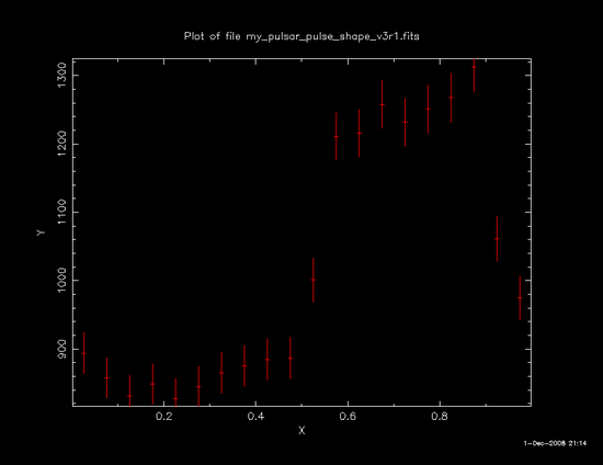
Now you have a pulse phase number [or a fractional part of &phi(ti) defined in the previous step] for each photon in your data. With those phase numbers, you can accumulate their distribution, or sub-select photons within a specific range of pulse phase.

In the following example, fhisto (FTOOLS) creates a folded light curve, or a pulse shape, which is a distribution of values in PULSE_PHASE column of the event file named my_pulsar_events_phase_v3.fits, assuming that the file has already been processed by gtpphase as described in Section 3, above: Calculate Pulse Phase for Each Photon. The distribution will be stored into a histogram with the bin size of 0.05 in phase for phase values ranging from 0.0 to 1.0, and written into an output FITS file named my_pulsar_pulse_shape.fits under the column names of X, Y, and Error.

Now you can display the pulse shape with your favorite plotting tool, such as fplot (FTOOLS, an example shown below) and fv (FTOOLS). You can also print the contents of the histogram in ASCII format by using fdump (FTOOLS).