Period Search
(gtpsearch Tutorial)
The gtpsearch tool searches for pulsations in data which is known or suspected to have a pulsation of a known approximate period or frequency.
Note: It is not useful for a so-called blind period search, in which data are examined for pulsations at any frequency.
Known Issues: When running gtpsearch multiple times using the GUI, plot windows from previous runs reappear after they are closed manually. Thus, there is no way to permanently close plot windows without exiting the GUI.
Prerequisites
- Event data file in FT1 format, also known as a photon data file. (See Extract LAT Data.)
- Orbit file to use for the barycentric correction
- Ephemeris information of suspected pulsation provided in one of the following forms:
- Manually input the source (pulsar) location (for the barycentric correction), pulse frequency or period, and related information
- Automatically extracted from a pulsar ephemerides database, available online.
Sample Files. To try the examples in this section, you can download the following fake data files:
| (1.9 MB) | ||
| (108 kB) | ||
| (248 kB) |
Note: The output of gtpsearch consists of text describing the result of the periodicity search and an optional plot. This tool also creates an output file when requested. The output file contains the result of computation, i.e., the search result in the text output and the data array to plot, for future reference.
| Also see: | Tutorial (popup) |
SciTools References (Popup) |
|
SciTools Reference Pages: If you want the SciTools Reference pages to open in a popup window, click on: Open Popup Reference Window.
How To Perform A Simple Search
Using A Pulsar Ephemerides Database File
Performing a period search is straight forward if the object of interest is listed in a pulsar ephemerides database file. The example below shows how to perform the test under these circumstances using the files described above. The time origin of periodicity test is taken to be the center of the observation. That means, if a pulsation is found, the pulse frequency should be interpreted as measured at the center of the observation (i.e., the time origin).
The command shown below produces the following output message that describes the search criteria and explains the search result.
A plot will also be produced which is similar to the following plot.
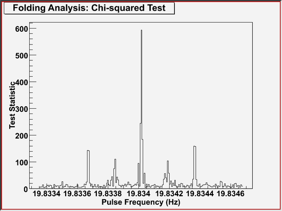
This plot very likely shows a pulsation consistent with the ephemeris found in the file.
Using Estimated Frequency Only
In practice, an ephemerides file which contains the object of interest may not be available. In this case, one may still proceed if one has an estimate for the frequency from some other source. Suppose the best known estimate for the frequency at 54368.11094817 MJD (TDB) were 19.8339 Hz. One could then run gtpsearch as follows.

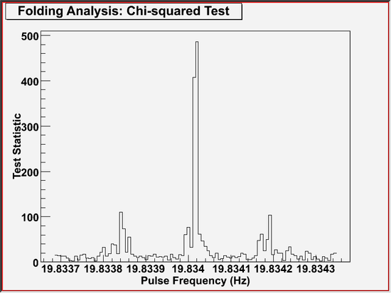
The result is similar to the first example, but the main peak in the plot is shifted to the right because the estimated frequency used for the search center was chosen to be noticeably lower than the peak frequency for demonstration purposes. The peak still occurs at the correct frequency, but the value of the statistic is lower because the trial frequencies are coarsely spaced on the natural frequency scale determined intrinsically by the data set.
Correcting For Known Frequency Variations
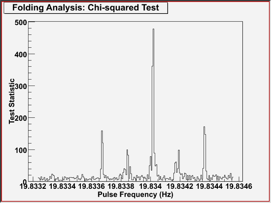
From the shape of the graph, it appears that there is a strong maximum with mainly symmetric side lobes. Encouraged by this result, one might run the tool again, using the position of the peak from the previous run as the central frequency. (The position of the peak is stated at the beginning of the tool output.) To zoom in on the peak more closely, the number of trials will be reduced to 100. In addition, the process of correcting for variations in the frequency known from other observations will be demonstrated. For this example, the frequency derivatives were taken from full independent analyses of ASCA data.
The effect of correcting for frequency variation was to increase the value of the maximum statistic, or the height of the main peak. Changing the central frequency brought the main peak back to the center of the graph. With the smaller number of trials, the second lobe on either side was cut off.
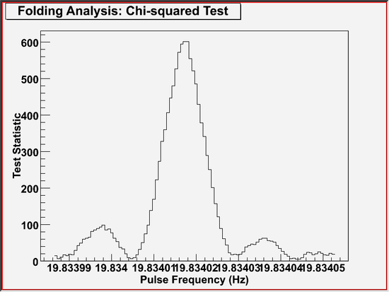
Looking For Precise Centroid Of The Peak
By decreasing the steps between subsequent trials, one can see the shape of the peak in a finer resolution.
Getting More Information on Computation
If gtpsearch is invoked with chatter parameter set to 4 or larger, it will display brief summaries of loaded ephemerides, arrival time corrections, and time systems being used, followed by a description of test condition and test result with periodgram data (i.e., a list of all trial frequencies and values of test statistic at the frequencies). This feature shows you additional information on computations being performed, which may help you understand the tool. Also, the extra information printed may contain a clue to diagnose certain types of problem. So, try a high chatter when you are unsure on the tool's behavior.
Going Beyond The Simple Case
How To Use Other Statistical Tests
In the examples above, the Chi-Squared statistic was used for purposes of finding the pulsation. The gtpsearch tool currently also supports the Z2n test, the Rayleigh test, and the H test. A full explanation of the strengths and weaknesses of these approaches is beyond the scope of this document; but in brief, the most effective test depends on the pulse shape. For the sample data used in this test, all the tests return similar results, so specific examples using the other tests will not be shown.Working In The Period Domain
The examples above all used inputs in the form of frequencies, and derivatives of frequencies. It is also possible to enter the input data as periods and derivatives of periods. These values are immediately converted to the frequency domain, and the search is still performed in the frequency domain. To enter period information instead, select PER for the ephemeris style. For example, the following input should produce the same plot as the example Using Estimated Frequency Only.
| Owned by: | Masaharu Hirayama hirayama@jca.umbc.edu |
| James Peachey James.Peachey-1@nasa.gov |
| Last updated by: Masaharu Hirayama 12/16/2008 |