Review: LAT Data Analysis Compare: pyLikelihood - Unbinned and Binned Analysis See: pyLikelihood Function Parameters: UnbinnedAnalysis Perform:
Also see: |
Run Prerequisite Science Tools (BinnedAnalysis)
Prerequisites
Procedure
Note: Steps 1 and 2, enable you to eliminate photons coming from the Earth limb by applying a zenith angle cut of 105o; gtmktime also updates the Good Time Intervals (GTIs) to match the FT2 data.
For a more detailed discussion, see Agreed procedures for data preparation: Removing Earth's Albedo and Correcting GTIs.
Note: gtltcube outputs an expCube.fits file, a HealPix table covering the full sky of the integrated livetime as a function.
- Create a source model XML file (using the Astro Data Viewer tool and the diffuse model recommend by the Diffuse Science Group).
1. Run gtselect |
Refer to: gtselect. |
- Run gtselect as follows:
chuckp@noric05 $ gtselect |
Note: Since we obtained our data from the Astro Data server and are only running gtselect to filter out any data greater than 105o, the maximum zenith angle, we could simply enter: Input FT1 file; Output FT1 file; radius of the new search region [180]; and maximum zenith angle value [105].
- Verify that the output file is now in your work directory.
2. Select GTIs (using gtmktime) |
|
Tip: Use gtvcut if you wish to view the Data SubSpace Keywords. (See gtvcut Help file; also see Data SubSpace Keywords.
3. Create Exposure Cube (using gtltcube) |
Refer to: gtltcube |
- Run gtltcube.
| chuckp@noric05 $ gtltcube Event data file[3C454_back-filtered.fits] Spacecraft data file[pyLike-ft2-30s.fits] Output file[3C454-expCube.fits] Step size in cos(theta) (0.:1.) [0.025] Pixel size (degrees)[1] Working on file pyLike-ft2.fits .....................! chuckp@noric05 $ |
- Verify that the output file is now in your work directory.
4. Create a 3D Counts Map (using gtbin CCube option)
- Run gtbin and select the CCUBE option.
Note: For the binned likelihood analysis, a three-dimensional counts map with an energy axis is required. Since the spectra of gamma-ray sources are expected to be fairly featureless and modeled rather simply, 20 logarithmically spaced energy bands over the range 30 MeV to 200 GeV is sufficient.
| chuckp@noric02 $ gtbin This is gtbin version v2r2p3 Type of output file (CCUBE|CMAP|LC|PHA1|PHA2) [CCUBE] Event data file name[3C454_back-filtered.fits] Output file name[3C454-CMap-3D.fits] Spacecraft data file name[pyLike-ft2-30s.fits] Size of the X axis in pixels[160] Size of the Y axis in pixels[160] Image scale (in degrees/pixel)[0.25] Coordinate system (CEL - celestial, GAL -galactic) (CEL|GAL) [CEL] First coordinate of image center in degrees (RA or galactic l)[343.6566] Second coordinate of image center in degrees (DEC or galactic b)[16.1494] Rotation angle of image axis, in degrees[0] Projection method e.g. AIT|ARC|CAR|GLS|MER|NCP|SIN|STG|TAN:[STG] Algorithm for defining energy bins (FILE|LIN|LOG) [LOG] Start value for first energy bin in MeV[100] Stop value for last energy bin in MeV[300000] Number of logarithmically uniform energy bins[20] chuckp@noric02 $ |
- Verify that the output file is now in your work directory.
5. Create Binned Exposure Map |
- Run gtexpcube.
chuckp@noric02 $ gtexpcube Cutoff used: 6.12303e-17 |
- Verify that the output file is now in your work directory.
Refer to: Also see: |
6. Create a Source Model XML File
(using Astro Data Viewer)
A. Copy the recommended XML model for the
Galactic diffuse emission:
- From your desktop, open a new .xml file in your XML editor.
- Refer to the Diffuse Model for Analysis of LAT Data page in Confluence, then click on the Web Access link near the top of the page.
The following page will be displayed in your browser:

- Click on the latest source_model (e.g., source_model_v02.xml at the time of this writing).
- An xml file be displayed in your browser; copy this file to your new xml file and save that file as 3C454-srcModel.xml.
- Note that there are two files referenced in this copy of the diffuse model that are listed in the diffuse model page shown in step 2, above. (At the time of this writing, those files were isotropic_iem_v02.txt and gll_iem_v02.fit.)
- Select and download these files, then copy them to your work directory on SLAC Public.
B. Generate an XML model for your Source (using the ASP Data Viewer)
and add it to the new source model file that you saved in step 4.
- Launch the ASP Data Viewer.
Select XML Source Model (upper right corner):
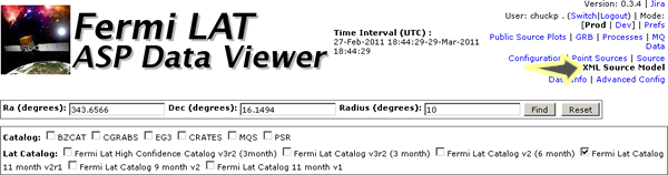
- Enter:
- Ra (degrees): 343.6566
- Dec (degrees): 16.1494
- Radius (degrees): 10
- Select Lat Catalog: Fermi Lat Catalog 11 month v1
- Click on the Find button.
The following sources will be displayed:

Observe that Source EMS1524 has an R.A. of 343.502 and a Dec of 16.1513.
- Make sure that all of the check boxes at the left have been selected; then, from the Spectrum List, select PowerLaw2 for each of them, and then click on the Generate XML button.
An xml file will be generated for the selected source(s).
- Copy this xml source model to the xml file you saved in step 4, above.
Your source model XML file should now look similar to this 3C454-srcModel.xml example.
Tip: Be sure that the first line in your xml file is <source_library title="source library">, and that the last line is </source_library>.
- Copy your XML source model file to your work directory on SLAC Public.
7. Compute Source Maps (using gtsrcmaps)
These are model count maps of each source, i.e., multiplied by exposure and convolved with the effective PSF.
If the binned exposure map file does not exist, then gtsrcmaps will compute an all-sky map with that name, using the energy bands of the 3D counts map. This exposure map can be reused for subsequent analyses of regions that cover the same time range and that use the same energy binning.
Since source map generation for the point sources is fairly quick, and maps for many point sources may take up a lot of disk space, it may be preferable to pre-compute the source maps for these sources at this stage. gtlike will compute these on the fly if they appear in the XML definition and a corresponding map is not in the source maps FITS file. To skip generating source maps for point sources, specify "ptsrc=no" on the command line when running gtsrcmaps.
chuckp@noric05 $ gtsrcmaps chuckp@noric05 $ ls |
- Verify that the output file is now in your work directory. Note that in this case it's not there, so we will rerun gtsrc again; this time without the Binned exposure map.
Note: If the binned exposure map file does not exist, then gtsrcmaps will compute an all-sky map with that name, using the energy bands of the 3D counts map. This exposure map can be reused for subsequent analyses of regions that cover the same time range and that use the same energy binning.
Since source map generation for the point sources is fairly quick, and maps for many point sources may take up a lot of disk space, it may be preferable to pre-compute the source maps for these sources at this stage. gtlike will compute these on the fly if they appear in the XML definition and a corresponding map is not in the source maps FITS file.
To skip generating source maps for point sources, specify gtsrcmaps ptsrc=no on the command line when running gtsrcmaps.
chuckp@noric05 $ gtsrcmaps ptsrc=no |
- Verify that the following files are now in your work directory: none and all-sky.
Note: When creating a python script to perform a binned analyis; as shown below, you will substitute these two files for 3C454-binned-expMap.fits and 3C454-srcMap.fits, respectively, when creating the BinnedObs constructor. For example,
likeObs = BinnedObs('3C454-srcMap.fits', '3C454-expCube.fits', '3C454-binned-expMap.fits', 'P6_V3_DIFFUSE')
will become:
likeObs = BinnedObs('all-sky', '3C454-expCube.fits', 'none', 'P6_V3_DIFFUSE')
You are now ready to perform a Binned pyLikelihood analysis.
| Last updated by: Chuck Patterson 08/17/2009 |