Likelihood Tutorial: Unbinned
Popup Windows: Examples: XML Model Definitions for Likelihood
Spatial Models: Related FTOOLS: Also see: |
Detection, flux determination, and spectral modeling of Fermi LAT sources is accomplished by a maximum likelihood optimization technique. This tutorial provides a step-by-step description for performing an unbinned likelihood analysis.
Unbinned vs Binned Likelihood
A binned analysis is also provided for cases where the unbinned analysis cannot be used: For example, since the memory required for the likelihood calculation scales with number of photons (and number of sources), memory usage can become excessive for long observations of complex regions, necessitating the use of a binned analysis, where the memory scales with then number of bins. For more detailed information, see the Likelihood Overview.
Prerequisites
- Event data file (often referred to as the FT1 file)
- Spacecraft data file (sometimes referred to as the FT2 file)
- Background models (Galactic diffuse emission model and extragalactic isotropic emission models)
Instructions for obtaining the data used in these examples are provided in the appropriate steps below.
Assumptions
The examples used in this exercise assume that you:
- are running in a bash shell on a SLAC Central Linux redhat5 64-bit machine. See Example: Setup (when running Science Tools on SLAC Central Linux).
- are using an SCons optimized redhat5-x86_64-64bit-gcc41 build for ScienceTools-xx-xx-xx.
- have set up a directory for your data (e.g., unbinned_likelihood_data) in your User Work Space (and that you will run the ScienceTools from within that directory).
Note: These files can be quite large, and you should not attempt to run them in your home directory.
- will use the data files provided (which are available for download).
You can also select your own data; see the LAT Data Access (green navbar) section of this workbook.
Steps
| It is assumed that you are running on SLAC Central Linux; if not, the setup instructions can readily be adapted to your environment. | |
| Since there is computational overhead for each event associated with each diffuse component, it is useful to filter out any events that are not within the extraction region used for the analysis. | |
| These simple FITS images let us inspect our data and help to pick out obvious candidate sources. | |
| This is needed for analyzing diffuse sources and derived absolute fluxes. | |
| Note: At the time this was written, November 03, 2010, the latest model was isotropic_iem_v02.txt. (See Fermi LAT U33 Disk Browser; also see Diffuse Model for Analysis of LAT Data confluence page.) | |
| The source model XML file contains the various sources and their model parameters to be fit using the gtlike tool. | |
Each event must have a separate response precomputed for each diffuse component in the source model. Skip this step unless you are using non-default background models. Each event must have a separate response precomputed for each diffuse component in the source model. |
|
| Fitting the data to the model can give flux, errors, spectral index, and more. | |
| These are used for point source localization and for finding weaker sources after the stronger sources have been modeled. | |
1. Setup
Be sure that the variation of ScienceTools you are using matches your operating system. The examples given in this exercise were running on a RHEL5-64 bit machine. If you are running on a SLAC Central Linux machine:
- Refer to the assumptions, above, then login to your home directory.
- If you have not already done so, create a directory (e.g., unbinned_likelihood_data) for your data in your User Work Space:
mkdir /afs/slac/g/glast/users/username/unbinned_likelihood_data
- Change to a redhat5 64-bit machine: ssh rhel5-64
- Setup your environment.
Tip: Use the emacs editor (available from the prompt by entering emacs) and create a setup script, e.g., setup_sciencetools-09-20-00. [See Example: Setup (when running Science Tools on SLAC Central Linux).]
Note: Since the data files can be very large, the example setup script assumes that you have already set up a data directory (e.g., likelihood_data) in your User Work Space where you will place your data (and from which you will run the science tools).
- Execute your setup script: source setup_sciencetools-09-20-00
- Change to your data directory: cd $My_data
Note: All of the following exercises assume that you are running the science tools from within your data directory.
2. Get the Data and Make Subselections from the Event Data.
- Get the Data. The original data selected for use in this analysis was:
- Search Center (RA, DEC) =(193.98, -5.82)
- Radius = 20 degrees
- Start Time (MET) = 239557417 seconds (2008-08-04 T15:43:37)
- Stop Time (MET) = 255398400 seconds (2008-02-04 T00:00:00)
- Minimum Energy = 100 MeV
- Maximum Energy = 100000 MeV
The following FT1 and FT2 files (which were used in this exercise) are provided:
- spacecraft.fits (61,926,593 KB, FT2 file)
- L100806104523E0D2F37E54_PH00.fits (81,335,430 KB, FT1 file)
- L100806104523EOD2F37E54_PH01.fits (54,674,985 KB, FT1 file)
You can download these files and place them in your work area, or you can obtain your own data [see the LAT Data Access (green navbar) section of this workbook].
Tip: These files can be quite large, and it is recommended that you create a data directory (e.g., likelihood_data) in your User Work Space, then create an environment variable (e.g., My_Data) that points to it. For example:
mkdir /afs/slac/g/glast/users/chuckp/likelihood_data
setenv My_Data /afs/slac/g/glast/users/<username>/likelihood_data
- Enter: cd $My_Data and place your data in this directory.
- Combine the FT1 events files. In order to combine the two events files for your analysis, you must first generate a text file listing the event data files to be included:
|
Note: This events.txt file will be used in place of the input fits filename when running gtselect. (See gtselect Help and gtselect Parameters.)
- Select photons. When analyzing a point source, it is recommended that you include events with a high probability of being photons.
gtselect high probability photons:To do this, use gtselect to perform cuts on the event class, keeping only event classes including and greater than (diffuse class):
prompt> gtselect evclsmin=3 evclsmax=4 |
Note: evclsmin and evclsmax are hidden parameters, so to use them for a cut, you must type them in the command line.
- Select the ROI. Perform a selection to the data you want to analyze.
gtselect ROI:For this example, we consider the diffuse class photons within a 20 degree region of interest (ROI) centered on the blazar 3C 279, and apply the gtselect tool to the data file as follows:
prompt> gtselect evclsmin=3 evclsmax=4 |
Notes:
- The FTOOLS syntax requires that you use an @ before the events.txt filename to indicate that this is a text file input rather than a fits file.
- In gtselect, there are hidden parameters that correspond to the event data file columns that may also be selected upon. However, as is customary with FTOOLS' hidden parameters, the typical user need not worry about them.
- gtselect writes descriptions of the data selections to a series of "Data Sub-Space" keywords in the EVENTS extension header. These keywords are used by the exposure-related tools and by gtlike for calculating various quantities, such as the predicted number of detected events given the source model.
These keywords must be same for all of the filtered event files considered in a given analysis. gtlike will check to ensure that all off the DSS keywords are the same in all of the event data files. For a discussion of the DSS keywords see the Data SubSpace Keywords page.
- The gtvcut tool can be used to view the DSS keywords in a given extension, where the EVENTS extension is assumed by default. (See gtvcut Help and gtvcut parameters.)
- We also selected the energy range and the maximum zenith angle value.
The Earth's limb is a strong source of background gamma rays, and we filter them out with a zenith angle cut; the value of 105 degrees is the cut most commonly used.
Example: 3C279_events_filtered.fits (optional).
- Determine the Good Time Intervals (GTIs). After the data selection is made, the GTIs in the event file should be recalculated to account for the zenith angle cut and to avoid time intervals for which the event data quality may be adversely affected by data processing issues, non-standard instrument configuration, or excessively large rocking angles.
The GTIs are used in the livetime and exposure calculations needed by the likelihood analysis tools. There are several options for calculating livetime depending on your observation type and science goals. For a detailed discussion of these options, see the Cicerone's Likelihood Livetime and Exposure.
To account for the cut on zenith angle, we use the gtmktime tool to exclude the time intervals where the zenith cut intersects the ROI. (See gtmktime Help and gtmktime parameters.) This is especially needed if you are studying a narrow ROI (with a radius of less than 20 degrees), as your source of interest may come quite close to the Earth's limb. To make this correction, you have to tell gtmktime to "Apply ROI-based zenith angle cut" by answering "yes" at the prompt. (See gtmktime example, below.)
gtmktime also provides an opportunity to select GTIs by filtering on information provided in the spacecraft file. (See the Cicerone's LAT File Types, Spacecraft File.) The current gtmktime filter expression recommended by the LAT team is
DATA_QUAL==1 && LAT_CONFIG==1 && ABS(ROCK_ANGLE)<52.
gtmktime example:This excludes time periods when some spacecraft event or data processing error has affected the quality of the data, ensures the LAT instrument was in normal science data-taking mode,and requires that the spacecraft be within the range of rocking angles used during nominal sky-survey observations.
The following is an example of running gtmktime for our analysis of the region surrounding 3C 279:
prompt> gtmktime |
Example: 3C279_events_gti.fits (optional).
- View DSS keywords. To view the DSS keywords in a given extension of a data file, use the gtvcut tool and review the data cuts on the EVENTS extension. (See gtvcut Help and gtvcut parameters.)
gtvcut:This provides a listing of the keywords reflecting each cut applied to the data file and their values, including the entire list of GTIs as shown in the example below:
prompt> gtvcut suppress_gtis=yes |
Note: This display includes the RA, Dec and ROI of the data selection, as well as: the energy range in MeV; the event class selection; the zenith angle cut applied; and it shows that the time cuts to be used in the exposure calculation are defined by the GTI table.
| Caution: Some of the Science Tools will not be able to run if you have multiple copies of the same DSS keyword. This can happen if the position used in extracting the data from the data server is different than the position used with gtselect. It is wise to review the keywords for duplicates before proceeding. If you do have keyword duplication, it is advisable to regenerate the data file with consistent cuts. |
3. Make Counts Maps from the Event Files.
Identify candidate sources. To identify candidate sources and to ensure that the field looks sensible, create a counts map of the region-of-interest (ROI), summed over photon energies.
Use the gtbin tool with the "CMAP" option (see gtbin Help and gtbin Parameters):
gtbin with "CMAP" option:prompt> gtbin |
Note: The last command launches the visualization tool ds9 and produces the following display:
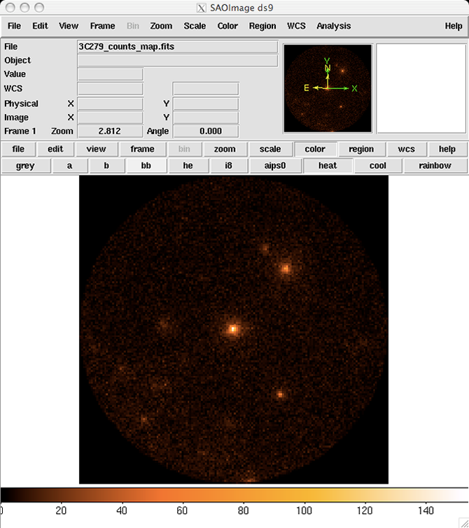 3C279_counts_map |
|
4. Make an Exposure Map
When creating an exposure map, it is important to note that the type of exposure map used by Likelihood differs from the usual notion of exposure maps (which are integrals of effective area over time) in that they include the effects of the PSF on the ROI data selection. (See gtexpmap Help and gtexpmap Parameters.)
The exposure calculation that Likelihood uses consists of an integral of the total response over the entire region-of-interest (ROI) data-space:
![]()
where primed quantities indicate measured energies, ![]() , and measured directions,
, and measured directions, ![]() . This exposure function can then be used to compute the expected numbers of events from a given source:
. This exposure function can then be used to compute the expected numbers of events from a given source:
![]()
where ![]() is the photon intensity from source i.
is the photon intensity from source i.
Since the exposure calculation involves an integral over the ROI, separate exposure maps must be made for every distinct set of DSS cuts. This is important if, for example, one wants to subdivide an observation to look for secular flux variations from a particular source or sources.
Note: To view the DSS keywords in a given extension of a data file, use the gtvcut tool and review the data cuts for the EVENTS extension. (See gtvcut Help and gtvcut parameters.)
The two tools needed for generating exposure maps are gtltcube and gtexpmap.
a. Use gtltcube to generate livetime cubes. gtltcube creates a HealPix table covering the full sky of the integrated livetime as a function of inclination with respect to the LAT z-axis. (See gtltcube Help and gtltcube Parameters.)gtltcube example:
prompt> gtltcube |
Notes:
- Values such as "0.1" for "Step size in cos(theta)" are known to give unexpected results. Use "0.09" instead.
- To download the the livetime cube generated for this analysis, click on: 3C279_ltcube.fits (optional).
Since gtltcube produces a FITS file covering the entire sky map, the output of this tool can be used for generating exposure maps for regions-of-interest in other parts of the sky that have the same time interval selections.
Caution: The livetime cube must be regenerated if you change any part of the time interval selection. This can occur by changing the start or stop time of the events, or simply by changing the ROI selection or zenith angle cut (as these produce an ROI-dependent set of GTIs from gtmktime). See:
Also see: |
b. Use gtexpmap to generate exposure maps. gtexpmap creates an exposure map based on the event selection used on the:
input photon file, and the
livetime cube.
Important! The exposure map must be recalculated if the ROI, zenith, energy selection or the time interval selection of the events is changed. (See gtexpmap Help and gtexpmap Parameters.)
prompt> gtexpmap |
Notes:
A 30 degree radius "source region" was chosen, even though an acceptance cone radius of 20 degrees was specified for gtselect. (See: What data should be used for source analysis?)
This is due to the size of the instrument point-spread function and is necessary to ensure that photons from sources outside the ROI are accounted for. Half-degree pixels are a nominal choice. (Smaller pixels should result in a more accurate evaluation of the diffuse source fluxes, but they will also make the exposure map calculation itself lengthier.)
The number of energies specifies the number of logarithmically spaced intervals bounded by the energy range given in the DSS keywords.
The last command shown above launches ds9 and produces the following display:
One image plane of the exposure map just created: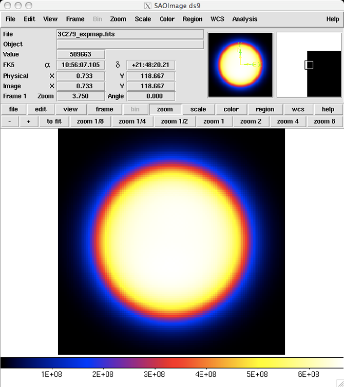 3C279_expmap |
5. Download the latest model for the isotropic background.
When using the latest Galactic diffuse emission model (e.g., gll_iem_v02.fit) in a likelihood analysis, also use the corresponding model for the Extragalactic isotropic diffuse emission (which includes the residual cosmic-ray background). At the time this was written, November 03, 2010, the latest model was isotropic_iem_v02.txt.
Download the following files from the Fermi LAT U33 Disk Browser:
- gll_iem_v02.fit
- isotropic_iem_v02.txt
Place these files in the same directory with your data.
Notes:
- For more information, refer to the Diffuse Model for Analysis of LAT Data page in confluence.
- The isotropic spectrum is valid only for the P6_V3_DIFFUSE response functions and only for data sets with front + back events combined.
6. Create a Source Model XML File.
The gtlike tool reads the source model from an XML file. (See gtlike Help and gtlike Parameters.) The source model can be created using the model editor tool or by editing the file directly within a text editor. Review the help information for the ModelEditor to learn how to run this tool.
Note: Given the dearth of bright sources in the extraction region we have selected, our source model file will be fairly simple, comprising only the Galactic and Extragalactic diffuse emission, and point sources to represent the blazars 3C 279 and 3C 273. For this example, use the diffuse background model as recommended by the LAT Team:
source model XML file:
Two types of sources can be defined:
- PointSource
- DiffuseSource.
Each type comprises a spectrum and a spatialModel component.
Model parameters are described by a set of attributes. The actual value of a given parameter that is used in the calculation is the value attribute multiplied by the scale attribute. The value attribute is what the optimizers see. Using the scale attribute is necessary to ensure that the parameters describing the objective function, -log(likelihood) for this application, all have values lying roughly within an order-of-magnitude of each other.
Each parameter has a range of valid values that can be specified.
The free attribute determines whether the parameter will be allowed to be fixed or free in the fitting process. Free flag attributes are currently disabled for spatial model parameters since fitting for these parameters has not been implemented (primarily due to the enormous overhead associated with computing the energy-dependent response functions for each source component).
The units for the spectral models are ![]() for point sources and
for point sources and ![]() for diffuse sources.
for diffuse sources.
Several spectral functions are available:
PowerLaw (see example XML Model Definition) This function has the form
![]()
where the parameters in the XML definition have the following mappings:
- Prefactor =

- Index =

- Scale =

BrokenPowerLaw (see example XML Model Definition)
![]()
where
- Prefactor =
- Index1 =

- Index2 =

- BreakValue =

PowerLaw2 (see example XML Model Definition)This function uses the integrated flux as a free parameter rather than the Prefactor:
![]()
where
- Integral =

- Index =
- LowerLimit =

- UpperLimit =

The UpperLimit and LowerLimit parameters are always treated as fixed, and as should be apparent from this definition, the flux given by the Integral parameter is over the range (LowerLimit, UpperLimit). Use of this model allows the errors on the integrated flux to be evaluated directly by likelihood, obviating the need to propagate the errors if one is using the PowerLaw form.
BrokenPowerLaw2 (see example XML Model Definition) Similar to PowerLaw2, the integral flux is the free parameter rather than the Prefactor:
![]()
where
![\[ \newcommand{\emin}{{E_{\rm min}}} \newcommand{\emax}{{E_{\rm max}}} \newcommand{\pfrac}[2]{\left(\frac{#1}{#2}\right)} \newcommand{\Int}{{\displaystyle\int}} N_0(N, E_{\rm min}, E_{\rm max}, \gamma_1, \gamma_2) = N \times \left\{\begin{array}{ll} \left[ \Int_\emin^\emax \pfrac{E}{E_b}^{\gamma_1} dE\right]^{-1} & \mbox{$\emax < E_b$}\\ \left[ \Int_\emin^\emax \pfrac{E}{E_b}^{\gamma_2} dE\right]^{-1} & \mbox{$\emin > E_b$}\\ \left[ \Int_\emin^{E_b} \pfrac{E}{E_b}^{\gamma_1} dE + \Int_{E_b}^\emax \pfrac{E}{E_b}^{\gamma_2} dE \right]^{-1} & \mbox{otherwise}\end{array}\right. \]](equations_04162008/form_31.png)
and
- Integral =
- Index1 =
- Index2 =
- BreakValue =
- LowerLimit =
- UpperLimit =
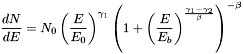
LogParabola (see example XML Model Definition) This is typically used for modeling Blazar spectra.
![]()
where
- norm =
- alpha =

- beta =

- Eb =
ExpCutoff (see example XML Model Definition) An exponentially cut-off power-law used for modeling blazar spectra subject to absorption by the extragalactic background light (EBL).
![\[ \newcommand{\pfrac}[2]{\left(\frac{#1}{#2}\right)} \frac{dN}{dE} = N_0 \times \left\{\begin{array}{ll} \pfrac{E}{E_0}^\gamma & \mbox{$E < E_b$}\\ \pfrac{E}{E_0}^\gamma \exp\left[ - ( (E - E_b)/p_1 + p_2\log(E/E_b) + p_3\log^2(E/E_b) ) \right] & \mbox{otherwise} \end{array}\right. \]](equations_04162008/form_35.png)
where
- Prefactor =
- Index =
- Scale =
- Ebreak =
- P1 =

- P2 =

- P3 =

BPLExpCutoff (see example XML Model Definition) An exponentially cut-off broken power-law.
![\[ \newcommand{\pfrac}[2]{\left(\frac{#1}{#2}\right)} \newcommand{\eabs}{{E_{\rm abs}}} \frac{dN}{dE} = N_0 \times \left\{\begin{array}{ll} \pfrac{E}{E_b}^{\gamma_1} & \mbox{$E < E_b$ and $E < \eabs$}\\ \pfrac{E}{E_b}^{\gamma_2} & \mbox{$E > E_b$ and $E < \eabs$}\\ \pfrac{E}{E_b}^{\gamma_1}\exp[-(E - \eabs)/p_1] & \mbox{$E < E_b$ and $E > \eabs$}\\ \pfrac{E}{E_b}^{\gamma_2}\exp[-(E - \eabs)/p_1] & \mbox{$E > E_b$ and $E > \eabs$}\end{array}\right. \]](equations_04162008/form_39.png)
where
- Prefactor =
- Index1 = =
- Index2 =
- BreakValue =
- Eabs =

- P1 =
Gaussian (see example XML Model Definition) A Gaussian function that can be used to model an emission line.
![]()
where
- Prefactor =
- Mean =

- Sigma =

ConstantValue (see example XML Model Definition) A constant-valued function, independent of energy.
![]()
where
- Value =
FileFunction (see example XML Model Definition) A function defined using an input ASCII file with columns of energy and differential flux values. The energy units are assumed to be MeV and the flux values are assumed to ![]() for a point source and
for a point source and ![]() for a diffuse source. The sole parameter is a multiplicative normalization.
for a diffuse source. The sole parameter is a multiplicative normalization.
![]()
where
- Normalization =
BandFunction (see example XML Model Definition) This function is used to model GRB spectra
![\[ \newcommand{\pfrac}[2]{{(#1/#2)}} \frac{dN}{dE} = N_0 \times \left\{\begin{array}{ll} \pfrac{E}{0.1}^\alpha \exp\left[-(E/E_p)(\alpha + 2)\right] & \mbox{if $E < E_p(\alpha - \beta)/(\alpha + 2)$}\\ \pfrac{E}{0.1}^\beta\left[\pfrac{E_p}{0.1} \frac{\alpha - \beta}{\alpha + 2}\right]^{\alpha - \beta} \exp(\beta - \alpha) & \mbox{otherwise} \end{array} \right. \]](equations_04162008/form_46.png)
where
- norm =
- alpha =
- beta =
- Ep =

- Scale =
PLSuperExpCutoff (see example XML Model Definition) For modeling pulsars.
![]()
where
- Prefactor =
- Index1 =
- Scale =
- Cutoff =

- Index2 =
SmoothBrokenPowerLaw (see example XML Model Definition)
where
- Prefactor =
- Index1 =
- Scale =
- Index2 =
- BreakValue =
- Beta =
Four spatial models are available:
- ConstantValue provides a constant value regardless of what argument value it takes. In the current context, ConstantValue is used to model the isotropic diffuse emission. As a function, however, ConstantValue is fairly general and can even be used in a spectral model; as it is when the spatial model is a MapCubeFunction.
- SpatialMap uses a FITS image file as a template for determining the distribution of photons on the sky. The EGRET diffuse model is given in the FITS file gas.cel, which describes the interstellar emission.
- MapCubeFunction used for diffuse sources that are modeled by a 3 dimensional FITS map (two sky coordinates and energy), thereby allowing arbitrary spectral variation as a function of sky position.
Note: The diffuse response depends on the spatial – and not the spectral – component of the background model. Changing the spectral form does not change the diffuse response by, for example, adding a modifying index to the galactic diffuse model, or changing the extragalactic isotropic model to use a power law spectrum.
Tip: Generating an Initial Source Model XML File. In practice, most people are using a python script (make1FGLXML.py) developed by Tyrel Johnson to generate an initial source model xml file based on the 1FGL catalog FITS file. This script:
You can validate your source model by loading it into ModelEditor, which will generate errors if the format is not correct for use with the Science Tools. |
7. Compute the Diffuse Source Responses.
Skip this step unless you are using non-default background models or IRFs. If you are using non-default background models or IRFs, you must perform this step.
The gtdiffrsp tool uses the name in the xml model to identify the existence of calculated diffuse response values. (See gtdiffrsp Help and gtdiffrsp Parameters.) This means that you need to use the provided diffuse files and match the naming scheme used for the diffuse components in the example above in order to take advantage of the precalculated diffuse response.
Note: If these quantities are not precomputed using the gtdiffrsp tool, gtlike will compute them at runtime. However, if multiple fits and/or sessions with the gtlike tool are anticipated, it is probably wise to precompute these quantities, as this step is very computationally intensive often taking ~hours to complete.
The source model XML file must contain all of the diffuse sources to be fit. The gtdiffrsp tool will add columns to the event data file for each diffuse source.
In the following example, the events file has been copied to a new file,
3C279_events_gti_altdiff.fits,
that will be used to calculate the alternate/non-standard diffuse response.
gtdiffrspprompt> gtdiffrsp |
Notes:
- The 3C279_events_gti_altdiff.fits file would now be available for performing a likelihood analysis if you wished to use the P6_V1_DIFFUSE instrument response function (IRF).
- A number of IRFs are distributed with the Fermi Science Tools. Some of these response functions, like P6_V3_DIFFUSE::FRONT, are designed to address only a subset of the events in the dataset, and thus would require you to make additional cuts before they could be used.
8. Run gtlike.
In the following example, most of the entries prompted for are fairly obvious. In addition to the various XML and FITS files, the user is prompted for a choice of IRFs, the type of statistic to use, the optimizer, and some output file names. (See gtlike Help and gtlike Parameters.)
gtlike:prompt> gtlike refit=yes plot=yes sfile=3C279_output_model.xml |
Note: gtobssim has the same option of generating events for these IRFs, and the choice used for gtlike must be the same as that chosen for gtobssim.
Statistics. The statistics available are:
- UNBINNED
In a standard unbinned analysis, such as the one described in this tutorial, the parameters for the spacecraft, event, and exposure files must be given.
- BINNED
In a binned analysis, the counts map and exposure hypercube files must be given, and the spacecraft, event, and exposure files are ignored.
Optimizers. There are five optimizers from which to choose:
- DRMNGB
- DRMNFB
- NEWMINUIT
- MINUIT
- LBFGS
Tip: Generally speaking, the faster way to find the parameters estimation is to:
- Use the DRMNGB (or DRMNFB) approach to find initial values.
- Then use MINUIT (or NEWMINUIT) to find more accurate results.
The application proceeds by reading in the spacecraft and event data, and if necessary, computing event responses for each diffuse source.
The output from our fit:Minuit did successfully converge. |
Note: Since we selected 'plot=yes' in the command line, a plot of the fitted data appears.
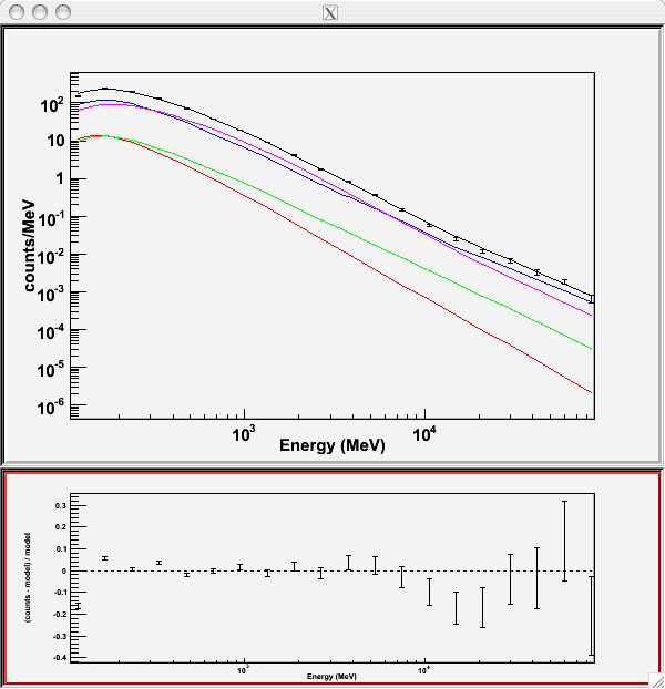 3C279_spectral_fit |
In the first plot:
The counts/MeV vs MeV are plotted. The points are the data, and the lines are the models. Error bars on the points represent sqrt(Nobs) in that band, where Nobs is the observed number of counts. The black line is the sum of the models for all sources. The colored lines follow the sources as follows:
- Black - summed model
- Red - first source in results.dat file (see below)
- Green - second source
- Blue - third source
- Magenta - fourth source
- Cyan - the fifth source
In this case:
- 3C273 = red
- 3C279 = green
- extragalactic background = blue
- galactic background = magenta
Note: If you have more sources, the colors are reused in the same order.
The second plot:
Gives the residuals between your model and the data.
Error bars here represent (sqrt(Nopbs))/Npred, where Npred is the predicted number of counts in each band based on the fitted model.
To assess the quality of the fit:
- Look first for the words at the top of the output "<Optimizer> did successfully converge." Successful convergence is a minimum requirement for a good fit.
- Next, look at the energy ranges that are generating warnings of bad fits. If any of these ranges affect your source of interest, you may need to revise the source model and refit.
- You can also look at the residuals on the plot (bottom panel). If the residuals indicate a poor fit overall, you should consider changing your model file, perhaps by using a different source model definition, and refit the data.
- If the fits and spectral shapes are good but could be improved, you may wish to simply update your model file to hold some of the spectral parameters fixed.
For example, by fixing the spectral model for 3C 273, you may get a better quality fit for 3C 279.
Closing the plot:
When you close the plot, you will be asked if you wish to refit the data.
Hitting 'return' will instruct the application to fit again.
We are happy with the result, so we type 'n' and end the fit.
Refit? [y] |
Results
When it completes, gtlike generates two standard output files:
- results.dat with the results of the fit, and
- counts_spectra.fits with predicted counts for each source for each energy bin.
The points in the plot above are the data points from the counts_spectra.fits file, while the colored lines follow the source model information in the results.dat file.
If you rerun the tool in the same directory, these files will be overwritten by default. Use the clobber=no option on the command line to keep from overwriting the output files.
Tip: The fit details and the value for the -log(likelihood) are not recorded in the automatic output files. You should therefore consider logging the output to a text file for your records by using "> fit_data.txt" (or something similar) with your gtlike command:
prompt> gtlike refit=yes plot=yes sfile=3C279_output_model.xml > fit_data.txt |
In the above example:
Output XML File. The 'sfile' parameter was used to request that the model results be written to an output XML file (3C279_output_model.xml). This file contains the source model results that were written to results.dat at the completion of the fit. If you have specified an output XML model file and you wish to modify your model while waiting at the 'Refit? [y]' prompt, you will need to copy the results of the output model file to your input model before making those modifications.
If you do not specify a source model output file with the 'sfile' parameter NO input xml file is written and nothing new is generated.
Scale. The results of the likelihood analysis have to be scaled by the quantity called "scale" in the XML model in order to obtain the total photon flux (photons cm-2 s-1) of the source. You must refer to the model formula of your source for the interpretation of each parameter. (See Create a Source Model XML File, above.)
In the example, the 'prefactor' of our power law model of 3C273 has to be scaled by the factor 'scale'=10-9. For example the total flux of 3C273 is the integral between 100 MeV and 100000MeV of:
Prefactor x scale x (E /100)index=(12.3809x10-9 * (E/100)-2.75107
Errors reported with each value in the results.dat file are 1-sigma estimates (based on the inverse-Hessian at the optimum of the log-likelihood surface).
Tip: To fetch the index and error from an unbinned analysis fit: model = like.model for 'self.sourceName', just substitute a string containing the exact source name in the model.xml file. For more "fetch" tips, see Fetching Fit Parameters. |
Other Useful Hidden Parameters
If you are scripting and wish to generate multiple output files without overwriting, the 'results' and 'specfile' parameters allow you to specify output filenames for the results.dat and counts_spectra.fits files, respectively.
9. Make Test-Statistic Maps.
Ultimately, one would like to find sources near the detection limit of the instrument.
Procedure Used in the analysis of EGRET data
The procedure used in the analysis of EGRET data was to:
- Model the strongest, most obvious sources (with some theoretical prejudice as to the true source positions, e.g., assuming that most variable high Galactic latitude sources are blazars, which can be localized by radio, optical, or X-ray observations).
- Then create 'Test-statistic maps' to search for unmodeled point sources.
These TS maps are created by moving a putative point source through a grid of locations on the sky and maximizing -log(likelihood) at each grid point with the other stronger — and presumably well-identified — sources included in each fit. New, fainter sources were then identified at local maxima of the TS map.
Using the gttsmap tool
The gttsmap tool can be run with or without an input source model. (See gttsmap Help and gttsmap Parameters.) However, for a useful visualization of the results of the fit, it is recommended you use the output model file from gtlike. (See gtlike Help and gtlike Parameters.)
Notes:
- The file must be edited so all parameters are fixed.
Otherwise gttsmap will attempt a refit of the entire model at every point on the grid.
- To see the field with the fitted sources removed (i.e. a residuals map), fix all point source parameters before running the TS map.
- To see the field with the fitted sources included, edit the model to remove all but the diffuse components.
- For residuals map: 3C279_output_model_resid.xml
- For sources TS map: 3C279_output_model_diffonly.xml
In both cases, the normalization parameters for the isotropic and galactic diffuse backgrounds should be left free.
- Running gttsmap is extremely time-consuming: the tool is performing a likelihood fit for all events at every pixel position.
One way to reduce the time required for this step is to use very coarse binning and/or a very small region.
In the following example, a TS map is run for the central 20x20 degree region of our data file, with .25 degree bins, resulting in 6400 maximum likelihood calculations.
Note: The run time for each of the maps discussed below was approximately four days.
Example of how to run the gttsmap tool to look for additional sources:prompt> gttsmap |
Resulting TS map: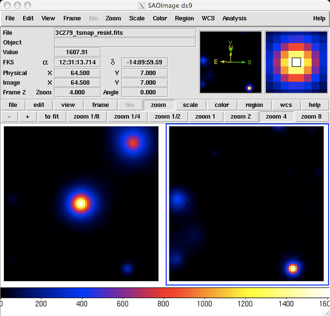 3C279_tsmap_tiled |
In the above example, the data set was small enough that an unbinned likelihood analysis was possible. With longer data sets, however, you may run into memory allocation errors, at which time it is necessary to move to binned analysis for your region.
Typical memory allocation error:gtlike(10869) malloc: *** mmap(size=2097152) failed (error code=12) |
If you encounter the error shown above, perform the Binned Likelihood Analysis.