.ipynb .pdf

repository suggest edit

Contents

Reproduce the cuts on generator level

The bhabha (2f_z_eehiq) sample would have been unmanagably large with the standard ILD production cuts. This higher cut point is indicated by the hiq suffix.

Here we look at the propagation of these cuts into quantities that can be constructed from the dst_merged.slcio files.

import awkward as ak
import matplotlib.pyplot as plt
import numpy as np
import uproot

from lcio_checks.mc.simulation import add_simulation_info
from lcio_checks.util import config
from lcio_checks.util import load_or_make

f = uproot.open(f"{config['data_dir']}/P2f_z_eehiq.root")["MyLCTuple"]
mc = f.arrays(filter_name="mc*", entry_stop=-1)
mc = add_simulation_info(mc)

Effect of generator level cuts on the Monte Carlo collections

Note: Due to beam overlay, there can be additional electrons and positrons in the detector/event.

el_in = mc[(mc.mcgst == 3) & (mc.mcpdg == 11)]
po_in = mc[(mc.mcgst == 3) & (mc.mcpdg == -11)]
el_out = mc[(mc.mcgst == 2) & (mc.mcpdg == 11)]
po_out = mc[(mc.mcgst == 2) & (mc.mcpdg == -11)]


def inv_mass_in_out_squared(p1, p2, t_channel=False):
    if t_channel:
        return (
            (p1.mcene - p2.mcene) ** 2
            - (p1.mcmox - p2.mcmox) ** 2
            - (p1.mcmoy - p2.mcmoy) ** 2
            - (p1.mcmoz - p2.mcmoz) ** 2
        )
    else:
        return (
            (p1.mcene + p2.mcene) ** 2
            - (p1.mcmox + p2.mcmox) ** 2
            - (p1.mcmoy + p2.mcmoy) ** 2
            - (p1.mcmoz + p2.mcmoz) ** 2
        )


ids_in_out = ak.argcartesian([el_out.mcpdg, el_in.mcpdg])
m_inv_in_out_squared = inv_mass_in_out_squared(
    el_out[ids_in_out.slot0], el_in[ids_in_out.slot1], t_channel=True
)
ids_ep = ak.argcartesian([el_out.mcpdg, po_out.mcpdg])
m_inv_ep = np.sqrt(
    inv_mass_in_out_squared(el_out[ids_ep.slot0], po_out[ids_ep.slot1], t_channel=False)
)

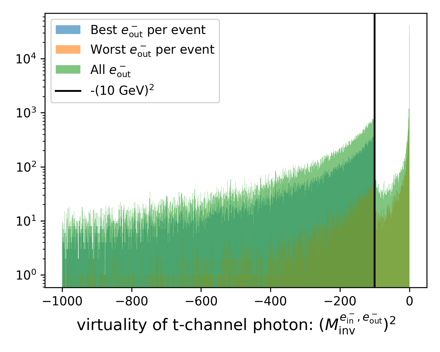
@load_or_make(["t_channel_virtuality_all.png"])
def t_channel_virtuality_all():
    fig, ax = plt.subplots(figsize=(5, 4))
    kw = dict(bins=np.linspace(-1000, 0, 1000), alpha=0.6)
    ax.hist(
        ak.min(m_inv_in_out_squared, axis=1),
        label=r"Best $e^-_\mathrm{out}}$ per event",
        **kw,
    )
    ax.hist(
        ak.max(m_inv_in_out_squared, axis=1),
        label=r"Worst $e^-_\mathrm{out}}$ per event",
        **kw,
    )
    ax.hist(ak.flatten(m_inv_in_out_squared), label=r"All $e^-_\mathrm{out}}$", **kw)
    ax.set_xlabel(
        r"virtuality of t-channel photon: $(M_\mathrm{inv}^{e^-_\mathrm{in}, e^-_\mathrm{out}})^2$",
        fontsize=13,
    )
    ax.axvline(-100, color="black", label="-(10 GeV)$^2$")
    ax.set_yscale("log")
    ax.legend()
    fig.tight_layout()
    return (fig,)


fig = t_channel_virtuality_all()

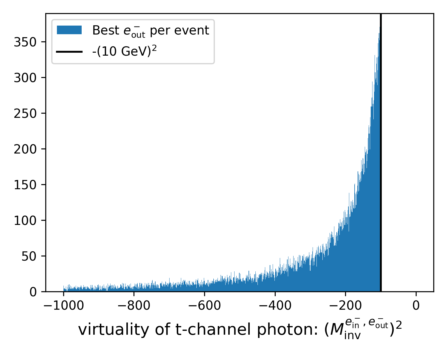
@load_or_make(["t_channel_virtuality.png"])
def t_channel_virtuality():
    fig, ax = plt.subplots(figsize=(5, 4))
    ax.hist(
        ak.min(m_inv_in_out_squared, axis=1),
        bins=np.linspace(-1000, 0, 1000),
        label=r"Best $e^-_\mathrm{out}}$ per event",
    )
    ax.set_xlabel(
        r"virtuality of t-channel photon: $(M_\mathrm{inv}^{e^-_\mathrm{in}, e^-_\mathrm{out}})^2$",
        fontsize=13,
    )
    ax.axvline(-100, color="black", label="-(10 GeV)$^2$")
    ax.legend()
    fig.tight_layout()
    return (fig,)


fig = t_channel_virtuality()

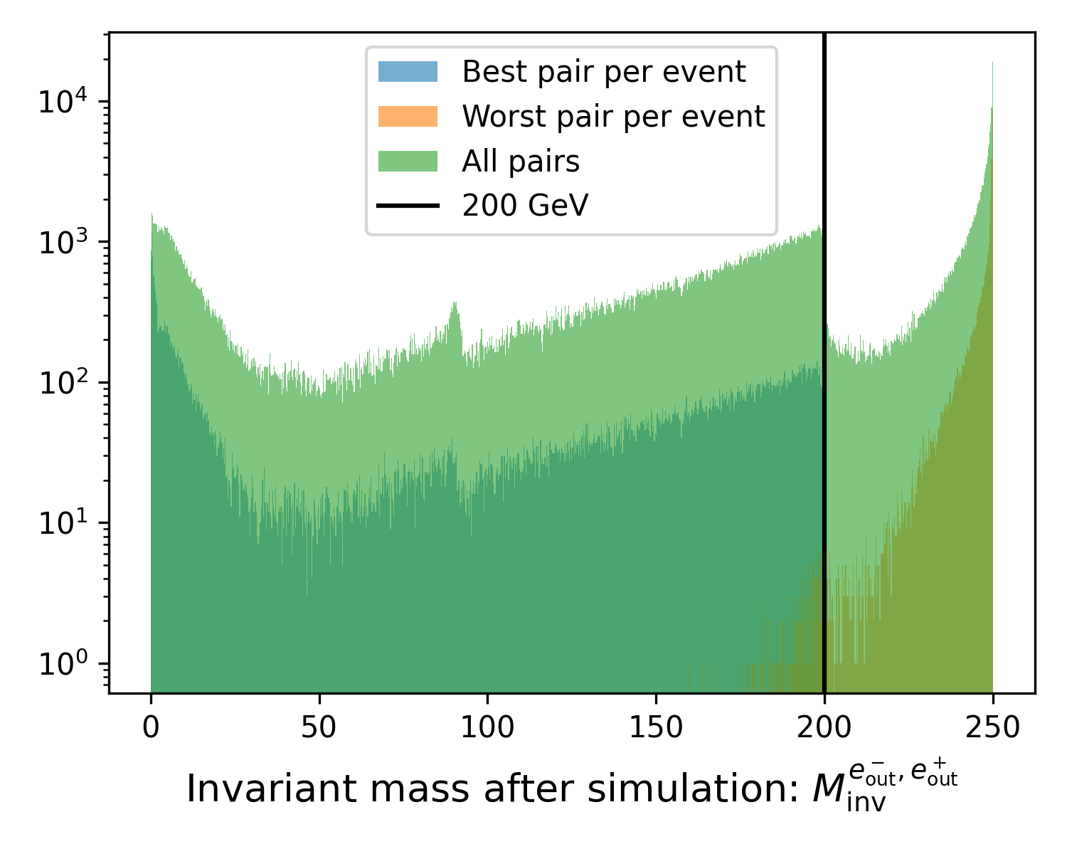
@load_or_make(["invariant_mass_simulation_all.png"])
def invariant_mass_simulation_all():
    fig, ax = plt.subplots(figsize=(5, 4))
    kw = dict(bins=np.linspace(0, 250, 1000), alpha=0.6)
    ax.hist(ak.min(m_inv_ep, axis=1), label="Best pair per event", **kw)
    ax.hist(ak.max(m_inv_ep, axis=1), label="Worst pair per event", **kw)
    ax.hist(ak.flatten(m_inv_ep), label="All pairs", **kw)
    ax.set_xlabel(
        r"Invariant mass after simulation: $M_\mathrm{inv}^{e^-_\mathrm{out}, e^+_\mathrm{out}}$",
        fontsize=13,
    )
    ax.axvline(200, color="black", label="200 GeV")
    ax.set_yscale("log")
    ax.legend()
    fig.tight_layout()
    return (fig,)


fig = invariant_mass_simulation_all()

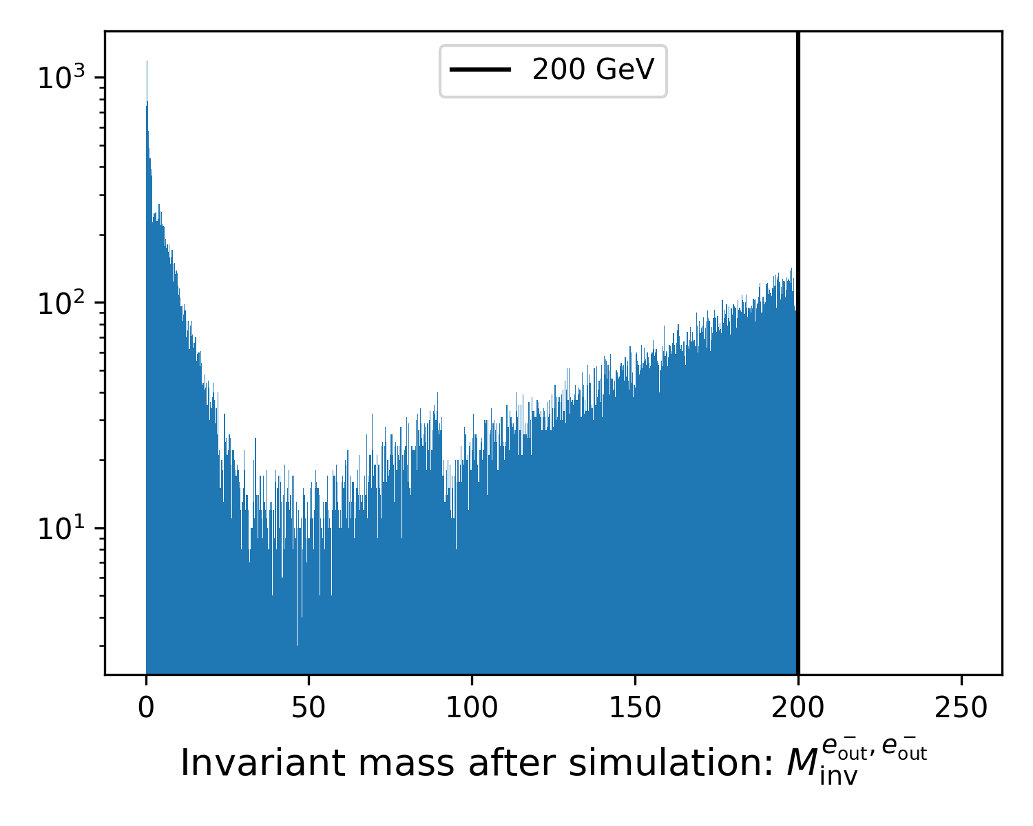
@load_or_make(["invariant_mass_simulation.png"])
def invariant_mass_simulation():
    fig, ax = plt.subplots(figsize=(5, 4))
    ax.hist(ak.min(m_inv_ep, axis=1), bins=np.linspace(0, 250, 1000))
    ax.set_xlabel(
        r"Invariant mass after simulation: $M_\mathrm{inv}^{e^-_\mathrm{out}, e^-_\mathrm{out}}$",
        fontsize=13,
    )
    ax.axvline(200, color="black", label="200 GeV")
    ax.set_yscale("log")
    ax.legend()
    fig.tight_layout()
    return (fig,)


fig = invariant_mass_simulation()

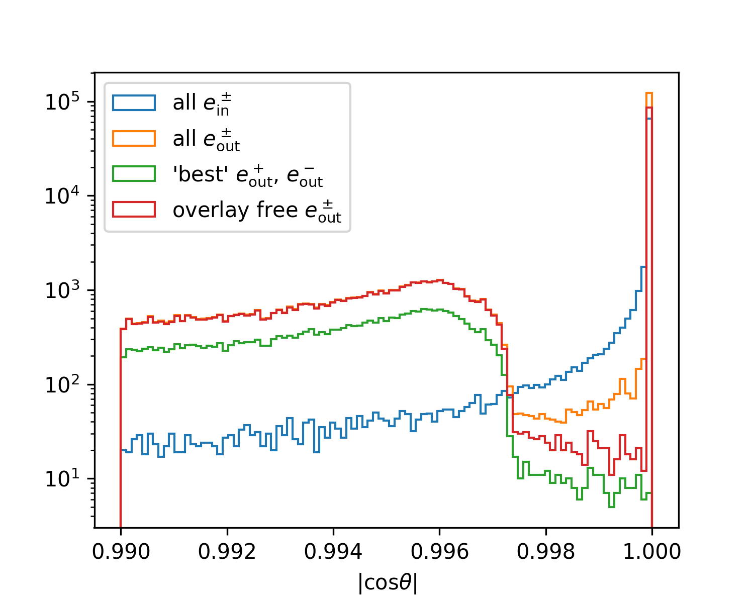
Consequences of these cuts: cos𝜃 spectrum

@load_or_make(["cos_theta_spectrum_simulation.png"])
def cos_theta_spectrum_simulation():
    kw = dict(bins=np.linspace(0.99, 1, 100), histtype="step")
    fig, ax = plt.subplots(figsize=(5, 4))
    for p1, p2, label, reducer in [
        (el_in, po_in, r"all $e^\pm_\mathrm{in}$", lambda x: ak.flatten(x)),
        (el_out, po_out, r"all $e^\pm_\mathrm{out}$", lambda x: ak.flatten(x)),
        (
            el_out,
            po_out,
            r"'best' $e^+_\mathrm{out}$, $e^-_\mathrm{out}$",
            lambda x: ak.min(x, axis=1),
        ),
        (
            el_out[~el_out.isOverlay],
            po_out[~po_out.isOverlay],
            r"overlay free $e^\pm_\mathrm{out}$",
            lambda x: ak.flatten(x),
        ),
    ]:
        x = np.concatenate(
            [reducer(np.abs(p1.mcmoz) / p1.mcene), reducer(np.abs(p2.mcmoz) / p2.mcene)]
        )
        ax.hist(x, label=label, **kw)
    ax.legend(loc="upper left")
    ax.set_yscale("log")
    ax.set_xlabel("|cos$\\theta$|")
    return (fig,)


fig = cos_theta_spectrum_simulation()

previous

Reconstructed particles

next

MC: Understand the generator status