Reconstructed particles
Contents
Reconstructed particles
import awkward as ak
import matplotlib.pyplot as plt
import numpy as np
import uproot

from lcio_checks.util import config, load_or_make

f = uproot.open(f"{config['data_dir']}/P2f_z_eehiq.root")["MyLCTuple"]
rc = f.arrays(filter_name="rc*", entry_stop=-1)
rp = rc[rc.rccid == 101]
RP Collections in the LCTuple
The reconstructed particles in the LCTuple rcXXX namespace are the combination of multiple LCIO collections.
The LCIO collection is tracked in the rccid field.
rccid |
LCIO collection |
|---|---|
101 |
PandoraPFOs |
102 |
BCALParticles |
103 |
PrimaryVertex_RP |
104 |
BuildUpVertex_RP |
105 |
BuildUpVertex_V0_RP |
Note: If you want to work with PFO objects I would observe in my detector, only use 101 and 102.
Counts in the sample per LCIO collection:
assert {101, 102, 103, 104, 105}.issuperset(np.unique(ak.flatten(rc.rccid)))

for cid, counts in zip(*np.unique(ak.flatten(rc.rccid), return_counts=True)):
    print(f"{cid}:{counts:>7d}")
print(f"\nNumber of events in the sample: {len(rc)}.")
101: 698556
103:  43199
104:    380
105:    145

Number of events in the sample: 43199.
Vertex collections
For now, we do not plan to study them further.
Let us only mention that all particles in these collection have their type defined as 3.
assert list(np.unique(ak.flatten(rc[rc.rccid > 102].rctyp).to_numpy())) == [3]
Particle types in PandoraPFOs
assert 102 not in np.unique(ak.flatten(rc.rccid))

import pandas as pd

uniq, counts = np.unique(
    np.abs(ak.flatten(rc[rc.rccid == 101].rctyp)), return_counts=True
)
df = pd.DataFrame(counts, index=uniq, columns=["counts"])
df.index.name = "Particle species"
df
| counts | |
|---|---|
| Particle species | |
| 11 | 94921 |
| 13 | 152 |
| 22 | 292288 |
| 211 | 234886 |
| 310 | 273 |
| 2112 | 75572 |
| 3122 | 464 |
A closer look into the Pandora PFOs
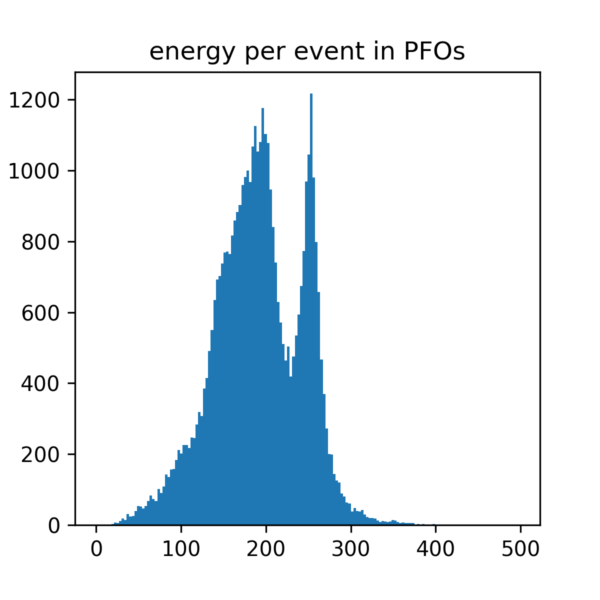
@load_or_make(["pfo_energy_per_event"])
def pfo_energy_per_event():
bins = np.arange(0, 501, 3)
fig, ax = plt.subplots(figsize=(4, 4))
ax.hist(ak.sum(rp.rcene, axis=1), bins=bins)
ax.set_title("energy per event in PFOs")
return (fig,)
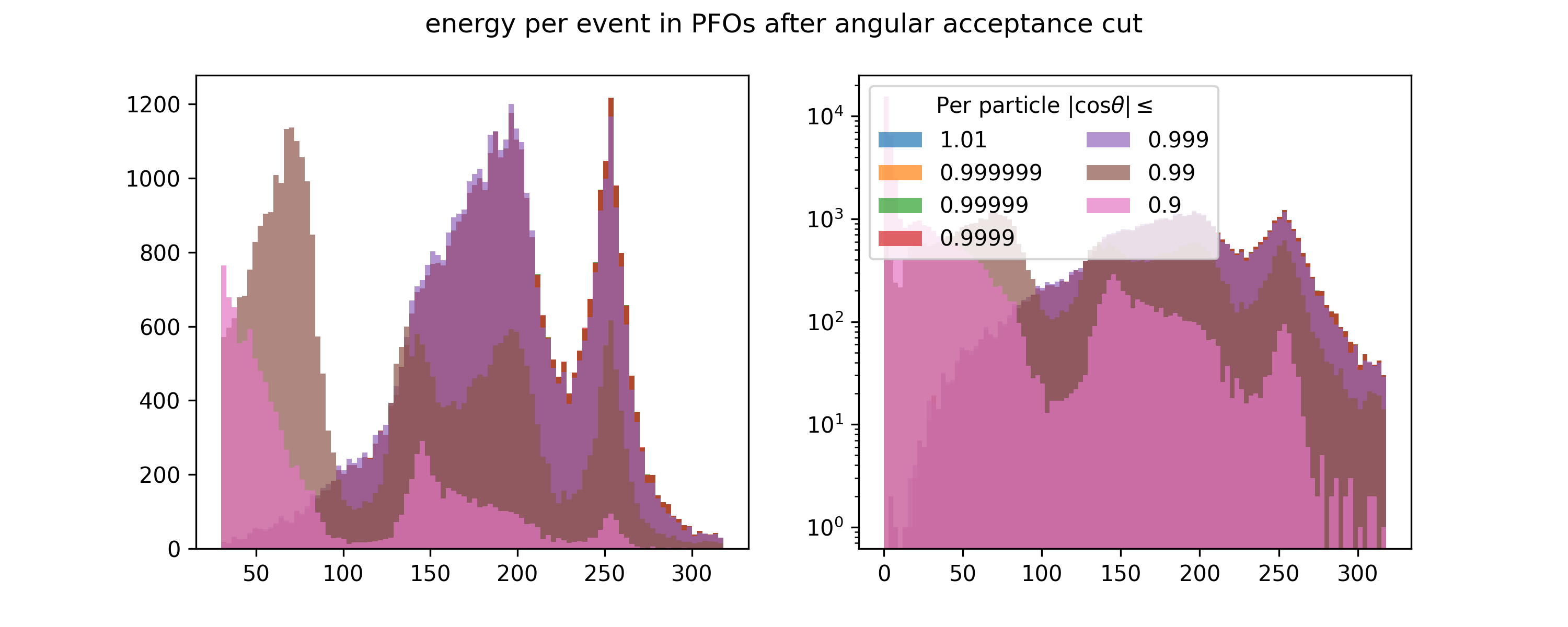
@load_or_make(["pfo_energy_per_event_after_acceptance"])
def pfo_energy_per_event_after_acceptance():
rcps = rp[rp.rcene != 0]
bins = np.arange(0, 321, 3)
fig, axs = plt.subplots(ncols=2, figsize=(10, 4))
for cos_theta in [1.01, 0.999999, 0.99999, 0.9999, 0.999, 0.99, 0.9]:
x = ak.sum(rcps[np.abs(rcps.rcmoz) / rcps.rcene < cos_theta].rcene, axis=1)
axs[0].hist(x, bins=bins[10:], label=str(cos_theta), alpha=0.7)
axs[1].hist(x, bins=bins, label=str(cos_theta), alpha=0.7)
axs[1].legend(title="Per particle |cos$\\theta$|$\\leq$", ncol=2)
axs[1].set_yscale("log")
fig.suptitle("energy per event in PFOs after angular acceptance cut")
return (fig,)
pfo_energy_per_event()
pfo_energy_per_event_after_acceptance();
Angular acceptance
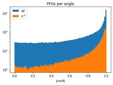
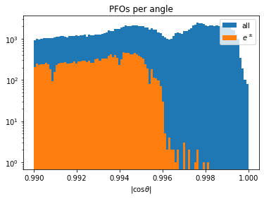
def particles_per_angle(rcps, bins):
    _, ax = plt.subplots(figsize=(6, 4))
    c_theta = np.abs(rcps.rcmoz) / rcps.rcene
    ax.hist(ak.flatten(c_theta), bins=bins, label="all")
    ax.hist(ak.flatten(c_theta[np.abs(rcps.rctyp) == 11]), bins=bins, label=r"$e^\pm$")
    ax.set_title("PFOs per angle")
    ax.set_xlabel("|cos$\\theta$|")
    ax.set_yscale("log")
    ax.legend()
    return ax


particles_per_angle(rp, bins=np.linspace(0, 1, 100))
particles_per_angle(rp, bins=np.linspace(0.99, 1, 100));