Likelihood Tutorial: Unbinned
In order to illustrate how to use the Likelihood software, this narrative gives a step-by-step description for performing an unbinned likelihood analysis, i.e., no set of data files is provided; rather you are expected to obtain the specific event and spacecraft data that you are interested in – see the Extract LAT Data Tutorial. However, if you go through the gtobssim tutorial first, you can essentially generate the same set of files for the likelihood analysis, providing you pick the same names for the gtobssim output. You can then follow along the likelihood tutorial exactly as written. |
|
|||
|
||||
Steps |
||||
| Since there is computational overhead for each event associated with each diffuse component, it is useful to filter out any events that are not within the extraction region used for the analysis. | ||||
| These simple FITS images let us see what we've got and help to pick out obvious candidate sources. | ||
| This is needed for analyzing diffuse sources. | ||
| The source model XML file contains the various sources and their model parameters to be fit using the gtlike tool. | ||
| Each event must have a separate response precomputed for each diffuse component in the source model. | ||
| These are used for point source localization and for finding weaker sources after the stronger sources have been modeled. |
1. Make Subselections from the Event Data.
For this tutorial, we will use data generated using gtobssim for a model comprising the Third EGRET (3EG) catalog sources and Galactic diffuse and extragalactic diffuse emission for a simulation time of one day. Since we have run gtobssim to create the event data, we have opted to write events from each component into separate event data files:
              glitch [40] [cillis]: ls -lrt *events_0000.fits
              -rw-r--r--  1 cillis lhea 138240 Feb 15 14:25 galactic_back_events_0000.fits
              -rw-r--r--  1 cillis lhea 161280 Feb 15 14:29 extragalactic_back_events_0000.fits
-rw-r--r-- 1 cillis lhea 34560 Feb 15 14:31 ptsrc_events_0000.fits |
We will consider data in the Virgo region within a 20 degree acceptance cone of the blazar 3C 279. Here we apply gtselect to the point source data; the same selections need to be applied to the files galactic_bck_events_0000.fits and extragalactic_bck_events_0000.fits:
     glitch [43] [cillis]: gtselect
     Input FT1 file [ptsrc_events_0000.fits] :
     Output FT1 file [ptsrc_events_filtered.fits] :
     RA for new search center (degrees) <0 - 360> [193.98] :
     Dec for new search center (degrees) <-90 - 90> [-5.82] :
     radius of new search region (degrees) <0 - 180> [20] :
     start time (MET in s) [252374400] :
     end time (MET in s) [254966400] :
     lower energy limit (MeV) [30] :
     upper energy limit (MeV) [200000] :
     Event classes (-1=all, 0=Front, 1=Back) <-1 - 4> [-1] :
     Done.
glitch [44] [cillis]: |
There are numerous hidden parameters that correspond to the event data file columns that may also be selected upon. However, as is customary with FTOOLS' hidden parameters, the typical user need not worry about them.
gtselect writes descriptions of the data selections to a series of "Data Sub-Space" keywords in the EVENTS extension header. These keywords are used by the exposure-related tools and by gtlike for calculating various quantities, such as the predicted number of detected events given the source model. These keywords must be same for all of the filtered event files considered in a given analysis. gtlike will check to ensure that all off the DSS keywords are the same in all of the event data files. For a discussion of the DSS keywords see the Data SubSpace Keywords page
The gtvcut tool can be used to view the DSS keywords in a given extension, where the EVENTS extension is assumed by default:
      glitch [45] [cillis]: gtvcut
      Input FITS file [ptsrc_events_filtered.fits] :
      Extension name [EVENTS] :
      DSTYP1: POS(RA,DEC)
      DSUNI1: deg
      DSVAL1: CIRCLE(193.98,-5.82,20)

      DSTYP2: TIME
      DSUNI2: s
      DSVAL2: TABLE
      DSREF2: :GTI

      GTIs:
      2.52374e+08  2.52461e+08

      DSTYP3: ENERGY
      DSUNI3: MeV
      DSVAL3: 30:200000
glitch [46] [cillis]: |
2. Make Counts Maps from the Event Files.
Next, we create a counts map file to visualize the extraction region we wish to fit. We create a file with the list of the three events files and then use the gtbin tool to create the count map: glitch [47] [cillis]: ls -1 *filtered.fits > eventFiles
glitch [48] [cillis]: gtbin
This is gtbin version v2r0p3
Type of output file <CCUBE|CMAP|LC|PHA1|PHA2> [CMAP] :
Event data file name [@eventFiles] :
Output file name [Virgo_Map.fits] :
Spacecraft data file name [../FT2/FT2.fits] :
Size of the X axis in pixels [200] :
Size of the Y axis in pixels [200] :
Image scale (in degrees/pixel) [0.25] :
Coordinate system (CEL - celestial, GAL -galactic) <CEL|GAL> [CEL] :
First coordinate of image center in degrees (RA or galactic l) [193.98] :
Second coordinate of image center in degrees (DEC or galactic b) [-5.82] :
Rotation angle of image axis, in degrees [0] :
Projection method <AIT|ARC|CAR|GLS|MER|NCP|SIN|STG|TAN> [AIT] :
glitch [49] [cillis]: ds9 Virgo_Map.fits |
The last command launches the visualization tool ds9 and produces this display:
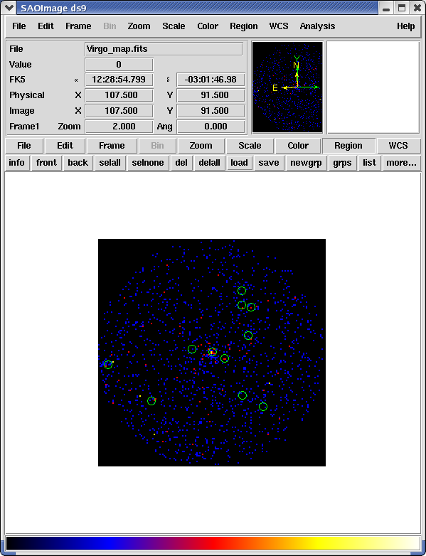
Virgo_map.fits
Here I have plotted as the green circles the locations of the 3EG point sources within 20 degrees of 3C 279.
3. Make an Exposure Map
We are now ready to create an exposure map. The type of exposure map used by Likelihood differs significantly from the usual notion of exposure maps, which are essentially integrals of effective area over time. The exposure calculation that Likelihood uses consists of an integral of the total response over the entire region-of-interest (ROI) data-space: ![]()
where primed quantities indicate measured energies, ![]() , and measured directions,
, and measured directions, ![]() . This exposure function can then be used to compute the expected numbers of events from a given source:
. This exposure function can then be used to compute the expected numbers of events from a given source:
![]()
where ![]() is the photon intensity from source i. Since the exposure calculation involves an integral over the ROI, separate exposure maps must be made for every distinct set of DSS cuts if, for example, one wants to subdivide an observation to look for secular flux variations from a particular source or sources.
is the photon intensity from source i. Since the exposure calculation involves an integral over the ROI, separate exposure maps must be made for every distinct set of DSS cuts if, for example, one wants to subdivide an observation to look for secular flux variations from a particular source or sources.
There are two tools needed for generating exposure maps. The first is gtltcube. This tool creates a HealPix table covering the full sky of the integrated livetime as a function of inclination with respect to the LAT z-axis. It is otherwise identical to the gtexpcube application in the map_tools package, except that gtltcube applies the time-range and GTI cuts specified in the DSS keywords of the filtered event files.
      glitch [50] [cillis]: gtltcube
      Event data file [ptsrc_events_0000.fits] :
      Spacecraft data file [../FT2/FT2.fits] :
      Output file [expCube.fits] :
      Step size in cos(theta) <0. - 1.> [0.025] :
      Pixel size (degrees) [1] :
      Working on file ../FT2/FT2.fits
      .....................!
glitch [51] [cillis]: |
Since gtltcube produces a FITS file covering the entire sky map, the output of this tool can be used for generating exposure maps for regions-of-interest in other parts of the sky that have the same time interval selections. Although the gtexpmap application (see below) can generate exposure maps for Likelihood without a livetime file, using one affords a substantial time savings.
Creating the exposure map using the gtexpmap tool, we have:
      glitch [52] [cillis]: gtexpmap
      The exposure maps generated by this tool are meant
      to be used for *unbinned* likelihood analysis only.
      Do not use them for binned analyses.
      Event data file [] : ptsrc_events_filtered.fits
      Spacecraft data file [] : ../FT2/FT2.fits
      Exposure hypercube file [] : expCube.fits
      output file name [] : expMap.fits
      Response functions [HANDOFF] :
      Radius of the source region (in degrees) [30] :
      Number of longitude points <2 - 1000> [120] :
      Number of latitude points <2 - 1000> [120] :
      Number of energies <2 - 100> [20] :
      Computing the ExposureMap using expCube.fits
      ....................!
glitch [53] [cillis]: |
Note that we have chosen a 30 degree radius "source region", while the acceptance cone radius specified for gtselect was 20 degrees. This is necessary to ensure that photons from sources outside the ROI are accounted for owing to the size of the instrument point-spread function. Half-degree pixels are a nominal choice; smaller pixels should result in a more accurate evaluation of the diffuse source fluxes but will also make the exposure map calculation itself lengthier. The number of energies specifies the number of logarithmically spaced intervals bounded by the energy range given in the DSS keywords. Here is one image plane of the exposure map we just created:
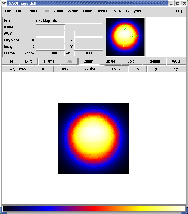
expMap.fits
4. Create a Source Model XML File.
The gtlike tool reads the source model from an XML file. Given the dearth of bright sources in the extraction region we have selected, our source model file will be fairly simple, comprising only the Galactic (using the one generated from gamma-ray intensities calculated by the GALPROP software) and extragalactic diffuse emission, and point sources to represent the blazars 3C 279 and 3C 273:
<?xml version="1.0" ?>
<source_library title="source library">
  <source name="Extragalactic Diffuse" type="DiffuseSource">
    <spectrum type="PowerLaw">
       <parameter free="1" max="100.0" min="1e-05" name="Prefactor" scale="1e-07" value="1.6"/>
       <parameter free="0" max="-1.0" min="-3.5" name="Index" scale="1.0" value="-2.1"/>
       <parameter free="0" max="200.0" min="50.0" name="Scale" scale="1.0" value="100.0"/>
     </spectrum>
     <spatialModel type="ConstantValue">
       <parameter free="0" max="10.0" min="0.0" name="Value" scale="1.0" value="1.0"/>
     </spatialModel>
   </source>
   <source name="Galpro Diffuse" type="DiffuseSource">
     <spectrum type="ConstantValue">
        <parameter free="0" max="10.0" min="0.0" name="Value" scale="1.0" value="1.0"/>
      </spectrum>
      <spatialModel file="$(EXTFILESSYS)/galdiffuse/GP_gamma.fits" type="MapCubeFunction">
        <parameter free="0" max="1000.0" min="0.001" name="Normalization" scale="1.0" value="1.0"/>
      </spatialModel>
   </source>
   <source name="3C 273" type="PointSource">
     <spectrum type="PowerLaw">
       <parameter free="1" max="1000.0" min="0.001" name="Prefactor" scale="1e-09" value="10"/>
       <parameter free="1" max="-1.0" min="-5.0" name="Index" scale="1.0" value="-2.1"/>
       <parameter free="0" max="2000.0" min="30.0" name="Scale" scale="1.0" value="100.0"/>
     </spectrum>
     <spatialModel type="SkyDirFunction">
       <parameter free="0" max="360" min="-360" name="RA" scale="1.0" value="187.25"/>
       <parameter free="0" max="90" min="-90" name="DEC" scale="1.0" value="2.17"/>
     </spatialModel>
   </source>
   <source name="3C 279" type="PointSource">
     <spectrum type="PowerLaw">
       <parameter free="1" max="1000.0" min="0.001" name="Prefactor" scale="1e-09" value="10"/>
       <parameter free="1" max="-1.0" min="-5.0" name="Index" scale="1.0" value="-2"/>
       <parameter free="0" max="2000.0" min="30.0" name="Scale" scale="1.0" value="100.0"/>
     </spectrum>
     <spatialModel type="SkyDirFunction">
       <parameter free="0" max="360" min="-360" name="RA" scale="1.0" value="193.98"/>
       <parameter free="0" max="90" min="-90" name="DEC" scale="1.0" value="-5.82"/>
     </spatialModel>
   </source>
</source_library> |
- Two types of sources can be defined, PointSource and DiffuseSource.
- Each type comprises a spectrum and a spatialModel component.
- Model parameters are described by a set of attributes. The actual value of a given parameter that is used in the calculation is the value attribute multiplied by the scale attribute. The value attribute is what the optimizers see. Using the scale attribute is necessary to ensure that the parameters describing the objective function, -log(likelihood) for this application, all have values lying roughly within an order-of-magnitude of each other.
- Each parameter has a range of valid values that can be specified.
- The free attribute determines whether the parameter will be allowed to be fixed or free in the fitting process. Free flag attributes are currently disabled for spatial model parameters since fitting for these parameters has not been implemented (primarily due to the enormous overhead associated with computing the energy-dependent response functions for each source component).
- The units for the spectral models are
 for point sources and
  for diffuse sources.
- Several spectral functions are available:
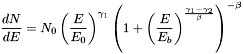
- PowerLaw (see example XML Model Definition) This function has the form
![\[ \frac{dN}{dE} = N_0 \left(\frac{E}{E_0}\right)^\gamma \]](equations_04162008/form_18.png)
where the parameters in the XML definition have the following mappings:
- Prefactor =

- Index =

- Scale =

- Prefactor =
- BrokenPowerLaw
(see example XML Model Definition)
![\[ \frac{dN}{dE} = N_0 \times\left\{\begin{array}{ll} (E/E_b)^{\gamma_1} & \mbox{if $E < E_b$}\\ (E/E_b)^{\gamma_2} & \mbox{otherwise} \end{array} \right. \]](equations_04162008/form_22.png)
where
- Prefactor =
- Index1 =

- Index2 =

- BreakValue =

- Prefactor =
- PowerLaw2 (see example XML Model Definition)This function uses the integrated flux as a free parameter rather than the Prefactor:
![\[ \frac{dN}{dE} = \frac{N(\gamma+1)E^{\gamma}} {E_{\rm max}^{\gamma+1} - E_{\rm min}^{\gamma+1}} \]](equations_04162008/form_26.png)
where
- Integral =

- Index =
- LowerLimit =

- UpperLimit =

The UpperLimit and LowerLimit parameters are always treated as fixed, and as should be apparent from this definition, the flux given by the Integral parameter is over the range (LowerLimit, UpperLimit). Use of this model allows the errors on the integrated flux to be evaluated directly by likelihood, obviating the need to propagate the errors if one is using the PowerLaw form. - Integral =
- BrokenPowerLaw2 (see example XML Model Definition) Similar to PowerLaw2, the integral flux is the free parameter rather than the Prefactor:
![\[ \frac{dN}{dE} = N_0(N, E_{\rm min}, E_{\rm max}, \gamma_1, \gamma_2) \times\left\{\begin{array}{ll} (E/E_b)^{\gamma_1} & \mbox{if $E < E_b$}\\ (E/E_b)^{\gamma_2} & \mbox{otherwise} \end{array} \right. \]](equations_04162008/form_30.png)
where
![\[ \newcommand{\emin}{{E_{\rm min}}} \newcommand{\emax}{{E_{\rm max}}} \newcommand{\pfrac}[2]{\left(\frac{#1}{#2}\right)} \newcommand{\Int}{{\displaystyle\int}} N_0(N, E_{\rm min}, E_{\rm max}, \gamma_1, \gamma_2) = N \times \left\{\begin{array}{ll} \left[ \Int_\emin^\emax \pfrac{E}{E_b}^{\gamma_1} dE\right]^{-1} & \mbox{$\emax < E_b$}\\ \left[ \Int_\emin^\emax \pfrac{E}{E_b}^{\gamma_2} dE\right]^{-1} & \mbox{$\emin > E_b$}\\ \left[ \Int_\emin^{E_b} \pfrac{E}{E_b}^{\gamma_1} dE + \Int_{E_b}^\emax \pfrac{E}{E_b}^{\gamma_2} dE \right]^{-1} & \mbox{otherwise}\end{array}\right. \]](equations_04162008/form_31.png)
and
- Integral =
- Index1 =
- Index2 =
- BreakValue =
- LowerLimit =
- UpperLimit =
- Integral =
- LogParabola (see example XML Model Definition) This is typically used for modeling Blazar spectra.
![\[ \newcommand{\pfrac}[2]{\left(\frac{#1}{#2}\right)} \frac{dN}{dE} = N_0\pfrac{E}{E_b}^{-(\alpha + \beta\log(E/E_b))} \]](equations_04162008/form_32.png)
where
- norm =
- alpha =

- beta =

- Eb =
- norm =
- ExpCutoff (see example XML Model Definition) An exponentially cut-off power-law used for modeling blazar spectra subject to absorption by the extragalactic background light (EBL).
![\[ \newcommand{\pfrac}[2]{\left(\frac{#1}{#2}\right)} \frac{dN}{dE} = N_0 \times \left\{\begin{array}{ll} \pfrac{E}{E_0}^\gamma & \mbox{$E < E_b$}\\ \pfrac{E}{E_0}^\gamma \exp\left[ - ( (E - E_b)/p_1 + p_2\log(E/E_b) + p_3\log^2(E/E_b) ) \right] & \mbox{otherwise} \end{array}\right. \]](equations_04162008/form_35.png)
where
- Prefactor =
- Index =
- Scale =
- Ebreak =
- P1 =

- P2 =

- P3 =

- Prefactor =
- BPLExpCutoff (see example XML Model Definition) An exponentially cut-off broken power-law.
![\[ \newcommand{\pfrac}[2]{\left(\frac{#1}{#2}\right)} \newcommand{\eabs}{{E_{\rm abs}}} \frac{dN}{dE} = N_0 \times \left\{\begin{array}{ll} \pfrac{E}{E_b}^{\gamma_1} & \mbox{$E < E_b$ and $E < \eabs$}\\ \pfrac{E}{E_b}^{\gamma_2} & \mbox{$E > E_b$ and $E < \eabs$}\\ \pfrac{E}{E_b}^{\gamma_1}\exp[-(E - \eabs)/p_1] & \mbox{$E < E_b$ and $E > \eabs$}\\ \pfrac{E}{E_b}^{\gamma_2}\exp[-(E - \eabs)/p_1] & \mbox{$E > E_b$ and $E > \eabs$}\end{array}\right. \]](equations_04162008/form_39.png)
where
- Prefactor =
- Index1 = =
- Index2 =
- BreakValue =
- Eabs =

- P1 =
- Prefactor =
- Gaussian (see example XML Model Definition) A Gaussian function that can be used to model an emission line.
![\[ \frac{dN}{dE} = \frac{N_0}{\sigma\sqrt{2\pi}} \exp\left[\frac{-( E - \bar{E} )^2}{2\sigma^2}\right] \]](equations_04162008/form_41.png)
where
- Prefactor =
- Mean =

- Sigma =

- Prefactor =
- ConstantValue (see example XML Model Definition) A constant-valued function, independent of energy.
![\[ \frac{dN}{dE} = N_0 \]](equations_04162008/form_44.png)
where
- Value =
- Value =
- FileFunction (see example XML Model Definition) A function defined using an input ASCII file with columns of energy and differential flux values. The energy units are assumed to be MeV and the flux values are assumed to for a point source and for a diffuse source. The sole parameter is a multiplicative normalization.
![\[ \frac{dN}{dE} = N_0\left.\frac{dN}{dE}\right|_{\rm file} \]](equations_04162008/form_45.png)
where
- Normalization =
- Normalization =
- BandFunction (see example XML Model Definition) This function is used to model GRB spectra
![\[ \newcommand{\pfrac}[2]{{(#1/#2)}} \frac{dN}{dE} = N_0 \times \left\{\begin{array}{ll} \pfrac{E}{0.1}^\alpha \exp\left[-(E/E_p)(\alpha + 2)\right] & \mbox{if $E < E_p(\alpha - \beta)/(\alpha + 2)$}\\ \pfrac{E}{0.1}^\beta\left[\pfrac{E_p}{0.1} \frac{\alpha - \beta}{\alpha + 2}\right]^{\alpha - \beta} \exp(\beta - \alpha) & \mbox{otherwise} \end{array} \right. \]](equations_04162008/form_46.png)
where
- norm =
- alpha =
- beta =
- Ep =

- Scale =
- norm =
- PLSuperExpCutoff (see example XML Model Definition) For modeling pulsars.
![\[ \newcommand{\pfrac}[2]{\left(\frac{#1}{#2}\right)} \frac{dN}{dE} = N_0 \pfrac{E}{E_0}^{\gamma_1} \exp\left(-\pfrac{E}{E_c}^{\gamma_2}\right) \]](equations_04162008/form_48.png)
where
- Prefactor =
- Index1 =
- Scale =
- Cutoff =

- Index2 =
- Prefactor =
- SmoothBrokenPowerLaw
(see example XML Model Definition)
where
- Prefactor =
- Index1 =
- Scale =
- Index2 =
- BreakValue =
- Beta =
- Prefactor =
- Four spatial models are available:
- SkyDirFunction describes a direction on the sky and is used only for point sources.
- ConstantValue provides a constant value regardless of what argument value it takes. In the current context, ConstantValue is used to model the isotropic diffuse emission. As a function, however, ConstantValue is fairly general and can even be used in a spectral model; as it is when the spatial model is a MapCubeFunction.
- SpatialMap uses a FITS image file as a template for determining the distribution of photons on the sky. The EGRET diffuse model is given in the FITS file gas.cel, which describes the interstellar emission.
- MapCubeFunction used for diffuse sources that are modeled by a 3 dimensional FITS map (two sky coordinates and energy), thereby allowing arbitrary spectral variation as a function of sky position.
5. Compute the Diffuse Source Responses.
If these quantities are not precomputed using the gtdiffrsp tool, then gtlike will compute them at runtime. However, if multiple fits and/or sessions with the gtlike tool are anticipated, it is probably wise to precompute these quantities. The source model XML file must contain all of the diffuse sources to be fit. The gtdiffrsp tool will add columns to the event data file for each diffuse source:
     glitch [66] [cillis]: gtdiffrsp
     Event data file [] : @eventFiles
     Spacecraft data file [] : ../FT2/FT2.fits
     Source model file [] : src_model.xml
     Response functions to use [HANDOFF] :
     adding source Extragalactic Diffuse
     adding source GalProp Diffuse
     Working on...
     extragalactic_back_events_filtered.fits.....................!
     galactic_back_events_filtered.fits.....................!
     ptsrc_events_filtered.fits......................!
glitch [67] [cillis]: |
Since 3C 273 and 3C 279 are point sources, diffuse responses are not calculated for these components.
6. Run gtlike.
We are now ready to run the gtlike application: glitch [94] [cillis]: gtlike refit=yes
Statistic to use <BINNED|UNBINNED> [UNBINNED] :
Spacecraft file [../FT2/FT2.fits] :
Event file [@eventFiles] :
Unbinned exposure map [expMap.fits] :
Exposure hypercube file [expCube.fits] :
Source model file [src_model.xml] :
Response functions to use [HANDOFF] :
Optimizer <DRMNFB|NEWMINUIT|MINUIT|DRMNGB|LBFGS> [MINUIT] :
|
Most of the entries prompted for are fairly obvious. In addition to the various XML and FITS files, the user is prompted for a choice of IRFs, the type of statistic to use, the optimizer, and some output file names.
gtobssim has the same option of generating events for these IRFs and the choice used for gtlike must be the same as that chosen for gtobssim.
The statistics available are:
- UNBINNED This is a standard unbinned analysis, described in this tutorial. If this option is chosen then parameters for the spacecraft file, event file, and exposure file must be given.
- BINNED This is a binned analysis, which is still in development. In this case, the Counts map file and Exposure hypercube file must be given. The spacecraft file, event file and exposure file are ignored in this case.
There are five optimizers from which to choose: DRMNGB, DRMNFB, NEWMINUIT, MINUIT and LBFGS. Generally speaking, the faster way to find the parameters estimation is to use DRMNGB (or DRMNFB) approach to find initial values and then use MINUIT (or NEWMINUIT) to find more accurate results.
If "Source model output file" is set to the same name as given to "Source model file" ("Virgo_model.xml" in this case), then that file will be overwritten with the latest fit. This is convenient as it allows the user to edit that file while the application is waiting at the "Refit? [y]" prompt so that parameters can be adjusted and set free or fixed. This would be similar to the use of the "newpar", "freeze", and "thaw" commands of XSPEC.
The "flux-style output file name" specifies the
destination of XML definitions of sources that can be used with gtobssim (or Gleam) to simulate an observation of the fitted source model.
The application proceeds by reading in the spacecraft and event data, and if necessary, computing event responses for each diffuse source.
Here is the output from our fit:
     **********
    **    1 **SET PRINT    0.000
    **********
    **********
    **    2 **SET NOWARN
    **********

    PARAMETER DEFINITIONS:
      NO.   NAME         VALUE      STEP SIZE      LIMITS
        1 'Prefactor '    10.000       1.0000        0.10000E-02   1000.0
        2 'Index     '   -2.1000       1.0000        -5.0000      -1.0000
        3 'Prefactor '    10.000       1.0000        0.10000E-02   1000.0
        4 'Index     '   -2.0000       1.0000        -5.0000      -1.0000
        5 'Prefactor '    1.6000       1.0000        0.10000E-04   100.00
    **********
    **    3 **SET ERR   0.5000
    **********
    **********
    **    4 **SET GRAD    1.000
    **********
    **********
    **    5 **MIGRAD    200.0       187.7
    **********
    MIGRAD MINIMIZATION HAS CONVERGED.

    MIGRAD WILL VERIFY CONVERGENCE AND ERROR MATRIX.

    FCN=   9365.969     FROM MIGRAD    STATUS=CONVERGED     74 CALLS       75 TOTAL
                        EDM=  0.49E-01    STRATEGY= 1      ERR MATRIX NOT POS-DEF

    EXT PARAMETER                APPROXIMATE        STEP         FIRST
    NO.   NAME        VALUE          ERROR          SIZE      DERIVATIVE
      1  Prefactor     5.9542        25.140       0.10063E-01    1.4074
      2  Index        -2.6775        3.1606       0.26481       0.34380
      3  Prefactor     10.082        6.9859       0.10063E-01   -1.9500
      4  Index        -2.2166       0.40695       0.12031       0.93418
      5  Prefactor     1.6766       0.20339       0.17127E-01    1.7086
                               ERR DEF= 0.500
    **********
    **    6 **HESSE
    **********
     FCN=   9365.969     FROM HESSE     STATUS=OK            33 CALLS      108 TOTAL
                        EDM=  0.15E-01    STRATEGY= 1      ERROR MATRIX ACCURATE

     EXT PARAMETER                                INTERNAL      INTERNAL
     NO.   NAME        VALUE          ERROR       STEP SIZE       VALUE
      1  Prefactor     5.9542        1.9595       0.19860E-03   -1.4163
      2  Index        -2.6775       0.29097       0.11153E-01   0.16198
      3  Prefactor     10.082        2.4143       0.79500E-03   -1.3697
      4  Index        -2.2166       0.14630       0.52846E-03   0.40250
      5  Prefactor     1.6766       0.10817       0.75720E-04   -1.3111
                               ERR DEF= 0.500
    Final values:
      Prefactor  = 5.95423
      Index      = -2.67746
      Prefactor  = 10.0816
      Index      = -2.21656
      Prefactor  = 1.67657
    Minuit fit quality: 3   estimated distance: 0.0151909
    Minuit parameter uncertainties:
      1  1.95967
      2  0.292031
      3  2.41451
      4  0.146457
      5  0.108174
    Computing TS values for each source (4 total)
    ....!

    3C 273:
    Prefactor: 5.95423 +/- 1.95967
    Index: -2.67746 +/- 0.292031
    Scale: 100
    Npred: 30.1573
    ROI distance: 10.4265
    TS value: 27.6889

    3C 279:
    Prefactor: 10.0816 +/- 2.41451
    Index: -2.21656 +/- 0.146457
    Scale: 100
    Npred: 65.5913
    ROI distance: 0
    TS value: 106.804

    Extragalactic Diffuse:
    Prefactor: 1.67657 +/- 0.108174
    Index: -2.1
    Scale: 100
    Npred: 462.92

    GalProp Diffuse:
    Value: 1
    Npred: 294.741
    WARNING: Fit may be bad in range [9176.18, 14251.4] (MeV)

    Total number of observed counts: 864
    Total number of model events: 853.41

    -log(Likelihood): 9365.968509

Refit? [y] |
At this point we can choose to edit the source model file, setting various spectral parameters free or fixed, and in the latter case, also setting them to some nominal value. For our refit, we fix the extragalactic diffuse component prefactors to their nominal values as follows:
   <source name="Extragalactic Diffuse" type="DiffuseSource">
    <spectrum type="PowerLaw">
       <parameter free="0" max="100.0" min="1e-05" name="Prefactor" scale="1e-07" value="1.6"/>
       <parameter free="0" max="-1.0" min="-3.5" name="Index" scale="1.0" value="-2.1"/>
       <parameter free="0" max="200.0" min="50.0" name="Scale" scale="1.0" value="100.0"/>
     </spectrum>
     <spatialModel type="ConstantValue">
       <parameter free="0" max="10.0" min="0.0" name="Value" scale="1.0" value="1.0"/>
     </spatialModel>
   </source>
   <source name="Galpro Diffuse" type="DiffuseSource">
     <spectrum type="ConstantValue">
        <parameter free="0" max="10.0" min="0.0" name="Value" scale="1.0" value="1.0"/>
      </spectrum>
      <spatialModel file="$(EXTFILESSYS)/galdiffuse/GP_gamma.fits" type="MapCubeFunction">
        <parameter free="0" max="1000.0" min="0.001" name="Normalization" scale="1.0" value="1.0"/>
      </spatialModel>
   </source>
|
We hit "return" to instruct the application to fit again. Here is the output:
   **********

   **********
   **    1 **SET PRINT    0.000
   **********
   **********
   **    2 **SET NOWARN
   **********

   PARAMETER DEFINITIONS:
      NO.   NAME         VALUE      STEP SIZE      LIMITS
       1 'Prefactor '    10.000       1.0000        0.10000E-02   1000.0
       2 'Index     '   -2.1000       1.0000        -5.0000      -1.0000
       3 'Prefactor '    10.000       1.0000        0.10000E-02   1000.0
       4 'Index     '   -2.0000       1.0000        -5.0000      -1.0000
   **********
   **    3 **SET ERR   0.5000
   **********
   **********
   **    4 **SET GRAD    1.000
   **********
   **********
   **    5 **MIGRAD    200.0       187.7
   **********
   MIGRAD MINIMIZATION HAS CONVERGED.

   MIGRAD WILL VERIFY CONVERGENCE AND ERROR MATRIX.

   MIGRAD MINIMIZATION HAS CONVERGED.

   MIGRAD WILL VERIFY CONVERGENCE AND ERROR MATRIX.

   FCN=   9365.962     FROM MIGRAD    STATUS=CONVERGED    109 CALLS      110 TOTAL
                       EDM=  0.84E-05    STRATEGY= 1      ERROR MATRIX ACCURATE

    EXT PARAMETER                                   STEP         FIRST
    NO.   NAME        VALUE          ERROR          SIZE      DERIVATIVE
     1  Prefactor     5.9173        1.9150       0.19991E-03  -0.80194E-01
     2  Index        -2.6853       0.29277       0.11447E-01  -0.21582E-01
     3  Prefactor     10.307        2.3627       0.79607E-03   0.37878E-01
     4  Index        -2.2315       0.14487       0.53265E-03   0.16953E-01
                               ERR DEF= 0.500
    **********
    **    6 **HESSE
    **********

    FCN=   9365.962     FROM HESSE     STATUS=OK            23 CALLS      133 TOTAL
                     EDM=  0.85E-05    STRATEGY= 1      ERROR MATRIX ACCURATE

     EXT PARAMETER                                INTERNAL      INTERNAL
     NO.   NAME        VALUE          ERROR       STEP SIZE       VALUE
      1  Prefactor     5.9173        1.8924       0.39982E-04   -1.4168
      2  Index        -2.6853       0.28938       0.45789E-03   -6.1252
      3  Prefactor     10.307        2.3557       0.15921E-03   -1.3674
      4  Index        -2.2315       0.14445       0.10653E-03   -5.8888
                               ERR DEF= 0.500
    Final values:
      Prefactor  = 5.917301433
      Index      = -2.685263371
      Prefactor  = 10.30702346
      Index      = -2.231545527
    Minuit fit quality: 3   estimated distance: 8.463995621e-06
    Minuit parameter uncertainties:
      1  1.892619146
      2  0.2904273627
      3  2.355889834
      4  0.1445955612
    Computing TS values for each source (4 total)
    ....!

    3C 273:
    Prefactor: 5.917301433 +/- 1.892619146
    Index: -2.685263371 +/- 0.2904273627
    Scale: 100
    Npred: 29.88982165
    ROI distance: 10.42650865
    TS value: 28.92086189

    3C 279:
    Prefactor: 10.30702346 +/- 2.355889834
    Index: -2.231545527 +/- 0.1445955612
    Scale: 100
    Npred: 66.34363994
    ROI distance: 0
    TS value: 112.6129873

    Extragalactic Diffuse:
    Prefactor: 1.6
    Index: -2.1
    Scale: 100
    Npred: 441.7781134

    GalProp Diffuse:
    Value: 1
    Npred: 294.7410871
    WARNING: Fit may be bad in range [174.543, 271.081] (MeV)
    WARNING: Fit may be bad in range [9176.18, 14251.4] (MeV)

    Total number of observed counts: 864
    Total number of model events: 832.7526621

    -log(Likelihood): 9365.961535

    Refit? [y]
    n
    Elapsed CPU time: 52.31
|
7. Make Test-Statistic Maps.
Ultimately, one would like to find sources near the detection limit of the instrument. The procedure used in the analysis of EGRET data was to model the strongest, most obvious sources (with some theoretical prejudice as to the true source positions, e.g., assuming that most variable high Galactic latitude sources are blazars which can be localized by radio, optical, or X-ray observations), and then create "Test-statistic maps" to search for unmodeled point sources. These TS maps are created by moving a putative point source through a grid of locations on the sky and maximizing -log(likelihood) at each grid point, with the other, stronger, and presumably well-identified sources included in each fit. New, fainter sources are then identified at local maxima of the TS map.Let's comment out 3C 273 from the source model XML file and see if we can find evidence for it in the data.
    glitch [103] [cillis]: gttsmap
    Event data file [eventFiles] :
    Spacecraft data file [../FT2/FT2.fits] :
    Exposure map file [expMap.fits] :
    Exposure hypercube file [expCube.fits] :
    Source model file [src_model.xml] :
    TS map file name [TsMap.fits] :
    Response functions to use [HANDOFF] :
    Optimizer <LBFGS|MINUIT|DRMNGB> [MINUIT] :
    Fit tolerance [1e-05] :
    x coordinate minimum <-360 - 360> [180] :
    x coordinate maximum <-360 - 360> [200] :
    Number of x coordinate points <2 - 200> [40] :
    y coordinate minimum <-90 - 90> [-10] :
    y coordinte maximum <-90 - 90> [10] :
    Number of y coordinate points <2 - 200> [40] :
    Coordinate system <CEL|GAL> [CEL] :
.....................! |
Here is the resulting TS map:
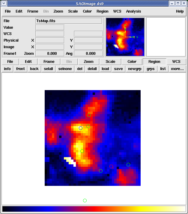
TsMap.fits
The various circles indicate the locations of the 3EG sources, all of which were included in the simulation. The red circle is 3C 279, the only source that was included in the TS map model; and the blue circle is at the location of 3C 273. Several other TS enhancements appear in the map and seem to be associated with other 3EG sources (green circles) that were not included in the the TS map model.
| Last updated by: Jim Chiang 06/09/2009 | ======= >>>>>>> 1.12 |