See pyLikelihood: Also see: |
Interactively Explore pyLikelihood Functions
You can perform a pyLikelihood analysis from the python prompt, which is useful in testing a new command and its parameters before incorporating it into a script file. Or, you may want to perform some functions interactively after performing an analysis (e.g., you may want to unset and change a fixed parameter).
For the purposes of continuity, we'll perform the same UnbinnedAnalysis that we performed in the pyLikelihood: UnbinnedAnalysis section of this tutorial, but this time from the python prompt.
Prerequisites
- Setup for SLAC Central Linux
- Get Data (using the new AstroServer)
- Run Prerequisite Science Tools (UnbinnedAnalysis)
Remember: We ran the "my_unbinned_analysis" script from our mypyLike work directory and used the following files:
- FT1.fits file - 3C454_back-filtered.fits
- FT2.fits file - pyLike-ft2-30s.fits
- expMap.fits - 3C454-expMap.fits
- expCube.fits - 3C454-expCube.fits
- IRFs - P6_V3_DIFFUSE
Create an UnbinnedObs object
- Log in to SLAC Central Linux and change to your work directory (e.g., mypyLike).
Note: If you are running on a Windows machine, use X-Win32 as your X server.
- Set up your SCons environment; see Setup SLAC Central Linux.
- At the prompt, enter: python.
- From the python prompt, import the data and analysis classes:
>>> from UnbinnedAnalysis import *
- Create an UnbinnedObs object; for example, the UnbinnedObs constructor is:
my_obs = UnbinnedObs('FT1.fits', 'FT2.fits', 'expMap.fits', 'expCube.fits', 'P6_V3_DIFFUSE'); so, from the python prompt, enter:
>>>likeObs = UnbinnedObs('3C454_back-filtered.fits', 'pyLike-ft2-30s.fits', '3C454-expMap.fits', '3C454-expCube.fits', 'P6_V3_DIFFUSE')
|


Create an Instance of UnbinnedAnalysis
- From the python prompt, enter:
>>>like = UnbinnedAnalysis(likeObs, srcModel="3C454-srcModel.xml")
The srcModel.xml is the xml file containing the model definition for Likelihood; see Create a Source Model XML File (using Astro Data Viewer).
|

View the UnbinneObs and UnbinnedAnalysis Classes
- To view the UnbinnedObs class, enter:
>>> print likeObs
Event file(s): 3C454_back-filtered.fits
Spacecraft file(s): pyLike-ft2-30s.fits
Exposure map: 3C454-expMap.fits
Exposure cube: 3C454-expCube.fits
IRFs: P6_V3_DIFFUSE
>>>
- To view the UnbinnedAnalysis class enter:
>>> print like
Event file(s): 3C454_back-filtered.fits
Spacecraft file(s): pyLike-ft2-30s.fits
Exposure map: 3C454-expMap.fits
Exposure cube: 3C454-expCube.fits
IRFs: P6_V3_DIFFUSE
Source model file: 3C454-srcModel.xml
Optimizer: Drmngb
>>>Note that the Optimizer is Drmngb, but we want MINUIT.
- Enter:
>>>like.optimizer="MINUIT"
Then enter:
- Enter:
>>>print like.fit(covar=True)
Note that the fit is: 4233.53736657
- Enter:
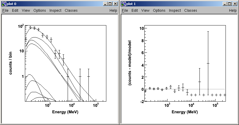
>>>like.plot()
>>> print like
Event file(s): 3C454_back-filtered.fits
Spacecraft file(s): pyLike-ft2-30s.fits
Exposure map: 3C454-expMap.fits
Exposure cube: 3C454-expCube.fits
IRFs: P6_V3_DIFFUSE
Source model file: 3C454-srcModel.xml
Optimizer: MINUIT
>>>
Note: If you're running on a Windows machine, be sure that you are using XWin-32 as your X Server.
- Enter:
>>> like.model
4233.53736657 |
Note: The columns are:
|
- You can change parameters using the index; for example (only), enter:
>>>like[33]=1.100
>>>like.fit(verbosity=0)
4233.5350369330818Note that the fit has changed from 4233.53736657 in step 10, above.
- Enter:
>>>like.oplot()

- Refer to pyLikelihood Attributes and Methods for additional functions that you can perform.
gt_apps
There are three key parts to gt_apps:
- gt_apps import command;
- gt_apps definitions; and the
- .run() command
For an example of a script using gt_apps, see: gt_apps python Script Used in Binaries RSP Analysis.
For more examples of more scripts, see Richard Dubois' confluence page "Scripts used in Binaries RSP Analysis".
Please note: In future versions of this tutorial, it is our intent to include additional links to useful scripts that have been developed by subject matter experts.
Later, it may be useful to consolidate these scripts into a user-friendly catalog.
| Owned by: | Jim Chiang |
| Last updated by: Chuck Patterson 04/01/2011 |