Likelihood Analysis from Python
|
Also see: |
Installation
To have access to likelihood analysis modules from Python, set your INST_DIR environment variable to point to the directory where you have installed your ScienceTools distribution, and source or execute the appropriate python_setup file in the pyLikelihood package. Following the example in the linux installation instructions, one would do:
noric07[jchiang] setenv INST_DIR ${HOME}/ST
noric07[jchiang] source ${INST_DIR}/pyLikelihood/v1r3p3/cmt/python_setup.csh
|
whereas under Windows, one might do:
C:\> set INST_DIR=%HOME%\ST C:\> %INST_DIR%\pyLikelihood\v0r0p1\Visual\python_setup.bat |
Note: For Windows, the python_setup.bat file lives in the Visual subdirectory, whereas for linux, the setup files, python_setup.[c]sh, live in the cmt subdirectory.
Run the python version that is in the distribution. For version v9r4p2 of the Science Tools is 2.5.1.
Package Description
Unbinned and binned analysis have been implemented in the UnbinnedAnalysis.py and BinnedAnalysis.py modules, respectively. Each module contains two classes: UnbinnedObs and UnbinnedAnalysis in the former, and BinnedObs and BinnedAnalysis in the latter.
The "Obs" classes differ in how they are constructed since the respective analyses require different sets of input data. Nonetheless, both implementations are intended to encapsulate the information associated with a specific observation. In this context, an observation is defined in terms of the extraction region in the data space of photon arrival time, measured energy, and direction. An observation also comprises ancillary information specific to the data selections such as the exposure information and the response functions to be used.
The signature of the UnbinnedObs constructor is:
class UnbinnedObs(object):
    def __init__(self, eventFile=None, scFile=None, expMap=None,
                 expCube=None, irfs='HANDOFF', checkCuts=True):
|
and its parameters are:
| eventFile | Event data file name(s), either a single file name or a tuple or list of file names. If given as a single file name, it can also be an ascii file of FITS file names. | |
| scFile | Spacecraft data file name(s). This can also be an ascii file of FITS file names. | |
| expMap | Exposure map (produced by gtexpmap). The geometry of this map matches that of the extraction region used to create the event files. | |
| expCube | Live-time cube (produced by gtltcube). This is an off-axis histogram of live-times at each point in the sky, partitioned as nested HealPix. | |
| irfs | Instrument response functions, e.g., HANDOFF |
|
| checkCuts | A flag used for debugging purposes. This should be set to True for a standard analysis. |
The BinnedObs constructor signature is:
class BinnedObs(object):
    def __init__(self, srcMaps, expCube, binnedExpMap=None, irfs='HANDOFF'):
|
and its parameters are:
| srcMaps | This is a counts map file with axes in position and energy and source map extensions created using gtsrcmaps. The counts map may be created with gtcmap. If one provides a counts map without a complete set of source map extensions, the BinnedAnalysis class will examine the model definition file and will compute source maps in memory for all the sources that do not have source maps in the counts map file. | |
| expCube | The live-time cube. | |
| binnedExpMap | Exposure map appropriate for binned likelihood analysis. This is optional. If it is not specified, then Likelihood will compute an appropriate map and output it as binned_exposure.fits. These exposure maps are matched to the geometry of the counts map in srcMaps. |
|
| irfs | Instrument response functions, e.g., HANDOFF |
Consult the unbinned and binned analysis tutorials for more detailed description of the inputs to these classes.
The "Analysis" classes have the same public interfaces and can therefore be used interchangably in scripts. The UnbinnedAnalysis constructor is defined as:
class UnbinnedAnalysis(AnalysisBase):
    def __init__(self, observation, srcModel=None,  optimizer='Minuit'):
|
and its parameters are:
| observation | An instance of the UnbinnedObs class. | |
| srcModel | Name of the XML file containing the source model definition. | |
| optimizer | Optimizer package to use: Minuit, NewMinuit Drmnfb, Drmngb, Lbfgs |
The BinnedAnalysis constructor is identical except that it takes an instance of BinnedObs as the observation object.
Factoring into separate analysis and observation classes affords flexibility in mixing and matching observations and models in a single Python session or script while preserving computational resources, so that one can do something like this:
>>> analysis1 = UnbinnedAnalysis(unbinnedObs, "model1.xml") >>> analysis2 = UnbinnedAnalysis(unbinnedObs, "model2.xml") |
Even though the two UnbinnedAnalysis instances access the same data in memory, distinct source models may be fit concurrently to those data without interfering with one another. This will be useful in comparing, via a likelihood ratio test, for example, how well one model compares to another.
Starting up from the Python command line
Here we perform an unbinned analysis. The steps that must be taken before proceeding, e.g., live-time, exposure and diffuse response calculations, are outlined in the unbinned analysis tutorial.First, we import the data and analysis classes:
>>> from UnbinnedAnalysis import * |
then we create an UnbinnedObs object:
>>> my_obs = UnbinnedObs(eventFiles, 'FT2.fits', expMap='expMap.fits', expCube='expCube.fits', |
Here, eventFiles is an ascii file containing the names of the event files:
glitch [43] [cillis]: cat eventFiles eg_dif_filtered.fits galdif_filtered.fits ptsrcs_filtered.fits glitch [44] [cillis]: |
One could also have entered in a tuple or list if file names or use glob to generate the list. For these data, the following are equivalent to the above:
>>> my_obs = UnbinnedObs(('eg_dif_filtered.fits', 'galdif_filtered.fits',
                          'ptsrcs_filtered.fits'),
                         'FT2.fits', expMap='expMap.fits',
                         expCube ='expCube.fits', irfs='HANDOFF')
|
OR
>>> my_obs = UnbinnedObs(glob.glob('*filtered.fits'), 'FT2.fits',
                         expMap='expMap.fits', expCube='expCube.fits',
                         irfs='HANDOFF')
|
One may omit all of the arguments in the UnbinnedObs class constructor, in which case a small GUI dialog is launched that allows one to browse the file system, use wild cards for specifying groups of files, etc.. So, entering:
>>> my_obs = UnbinnedObs() |
launches this dialog:
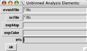
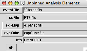
The buttons on the left will open file dialog boxes using the value shown in the text entry fields as a filter. One can include wild cards or comma-separated lists of files in the text entry field. Setting the entries as follows will create an UnbinnedObs object equivalent to the previous examples:
Now we are ready to create an instance of UnbinnedAnalysis:
>>> analysis = UnbinnedAnalysis(my_obs, "srcModel.xml") |
Here srcModel.xml is the xml file containing the model definition for Likelihood.
Just as with the UnbinnedObs class, a small GUI is provided that allows one to browse the file system in case one omits the name of the model XML file. For example:
>>> analysis = UnbinnedAnalysis(my_obs) |
launches:

The UnbinnedObs and UnbinnedAnalysis classes both have been implemented to allow one to see easily what data these objects comprise:
|
Starting from a Python Script
It is convenient to prepare a script that creates the UnbinnedObs and UnbinnedAnalysis objects with the proper parameter values so that analysis of the data may be easily revisited in separate sessions:
|
This just needs to be imported at the Python prompt:
>>> from my_analysis import * |
Viewing and Setting Parameters, Plotting, Fitting, etc.
Python provides various means of introspection. For example, the dir command shows an object's attributes:
>>> dir(like) ['Ts', '_Nobs', '__call__', '__class__', '__delattr__', '__dict__', '__doc__', |
The objects themselves may also offer introspection. Both UnbinnedAnalysis and BinnedAnalysis objects have a model attribute that allows one to view and manipulate the current state of the various fit parameters.
To view the current model parameters, do:
>>> like.model 3C 273 Spectrum: PowerLaw 0 Prefactor: 1.000e+01 0.000e+00 1.000e-03 1.000e+03 ( 1.000e-09) 1 Index: -2.100e+00 0.000e+00 -5.000e+00 -1.000e+00 ( 1.000e+00) 2 Scale: 1.000e+02 0.000e+00 3.000e+01 2.000e+03 ( 1.000e+00) fixed 3C 279 Spectrum: PowerLaw 3 Prefactor: 1.000e+01 0.000e+00 1.000e-03 1.000e+03 ( 1.000e-09) 4 Index: -2.000e+00 0.000e+00 -5.000e+00 -1.000e+00 ( 1.000e+00) 5 Scale: 1.000e+02 0.000e+00 3.000e+01 2.000e+03 ( 1.000e+00) fixed Extragalactic Diffuse Spectrum: PowerLaw 6 Prefactor: 1.600e+00 0.000e+00 1.000e-05 1.000e+02 ( 1.000e-07) 7 Index: -2.100e+00 0.000e+00 -3.500e+00 -1.000e+00 ( 1.000e+00) fixed 8 Scale: 1.000e+02 0.000e+00 5.000e+01 2.000e+02 ( 1.000e+00) fixed GalProp Diffuse Spectrum: ConstantValue 9 Value: 1.000e+00 0.000e+00 0.000e+00 1.000e+01 ( 1.000e+00) fixed >>> |
The columns are:
- parameter index
- parameter name
- parameter value
- error estimate (zero before fitting)
- lower bound
- upper bound
- parameter scaling (in parentheses)
- fixed (or not)
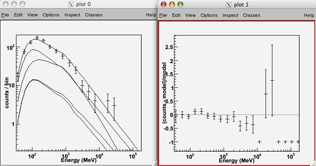
By default, the plot() method uses pyROOT to create counts spectra plots for comparing the model fits to the data. The following creates two plot windows, one for the counts spectra and one for the fractional residuals of the fit:
>>> like.plot() |
One can set parameter values using the index:
>>> like[6] = 1.595 |
optimizer::Parameter member functions are automatically dispatched to the underlying C++ class from Python so that one can set the "free" flag, set the bounds, and the scale factor
|
Now, perform a fit, suppressing Minuit's screen output; the resulting value -log(Likelihood) is returned:
>>> like.fit(verbosity=0) 9365.6790299170352 |
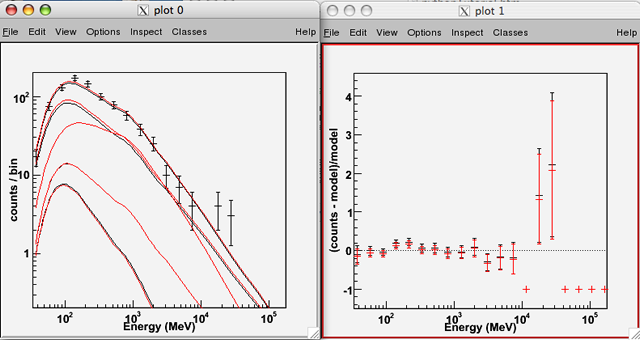
Overplot the new result in red, the default:
>>> like.oplot() |
The logLike attribute is a Likelihood::LogLike object, and so its member functions are exposed as Python methods:
|
Owned by: Jim Chiang
| Last updated by: Jim Chiang 09/29/2008 |