To get GBM Data, go to:
For information on GBM data:
For information on GBM instrument:
Also see:
|
GBM Gamma-ray Burst Analysis
This section provides the information needed to obtain the GBM data and understand how the data is organized, as well as a step-by-step example of using the gtbin and gtbindef tools, the FTOOLS, and the X-Ray Spectral Fitting Package (Xspec) to analyze GBM Gamma-Ray Burst observations.
Prerequisites
Assumptions
- Basic familiarity with XSPEC is assumed.
Performing a GBM Gamma-Ray Burst Analysis
The following is an example of how to perform a GRB analysis using gtbin, gtbindef, and some FTOOLS.
- Get the data. Go to the HEASARC Browse page.
(For this example the analysis, GRB080730520 data was used.)
Refer to Help: Browse Interface for GBM data.
- Examine "tcat" file. Identify the tcat file, and examine its contents using fdump; for example:
fdump glg_tcat_all_bn080730520.fit
|
This will provide useful information such as which detectors triggered for this burst:
DET_MASK= '110000001100' / Triggered detectors: (0-11) |
- Create light curve. Run gtbin on the time-tagged event (tte) data for one of the triggered detectors and examine the burst light curve for that detector:
prompt> gtbin
This is gtbin version v2r0p3
Type of output file (CCUBE|CMAP|LC|PHA1|PHA2) [LC]
Event data file name[glg_tcat_all_bn080730520.fit] glg_tte_n9_bn080730520.fit
Output file name[glg_tcat_all_bn080730520.lc] glg_tte_n9_bn080730520.lc
Spacecraft data file name[NONE]
Algorithm for defining time bins (FILE|LIN|SNR) [LIN]
Start value for first time bin in MET[INDEF]
Stop value for last time bin in MET[INDEF]
Width of linearly uniform time bins in MET[0.25] |
Notes:
- LC for 'Type of output file' indicates that you want to create a lightcurve.
- LIN for 'Algorithm for defining time bins' indicates that you want a linear time grid. The width of the time bins is the last parameter entered.
- Start and stop times are in Mission Elapsed Time; INDEF causes the program to use tstart and tstop of the original event.
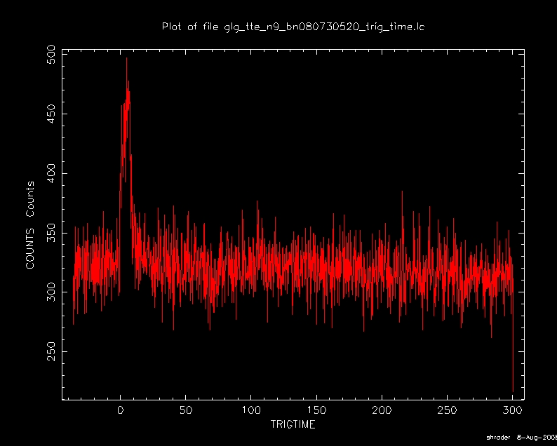
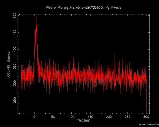
- Plot shifted light curve. To plot the light curve, shifted so that the trigger time is at t=0 fcal, first enter:
fcalc infile=glg_tte_n9_bn080730520.lc
outfile=glg_tte_n9_bn080730520_trig_time.lc
clname=TRIGTIME expr="Time-239113756.403240" |
Then plot the light curve using fplot:
fplot
infile=glg_tte_n9_bn080730520_trig_time.lc
xparm=TRIG_TIME
yparm=COUNTS
device="/Xw" |
Note: The interactive utility, Fv , is a more powerful alternative to fplot. (See Fv: The interactive FITS File Editor.)
For example, using fv, you can use the calculator function (in the 'tools' pull down menu of the 'summary' window of the extension with the quantities you want to plot) to define a new time variable equal to the time minus the trigger time. Then you can plot other variables vs. this new time variable.
And, when plotting quantities vs. time, you can subtract the trigger time from the time variable in the windows where the quantities to be plotted are specified.
- Using gtbindef. In this case, the burst lasts from about 0-12 seconds. Therefore, we'll use that range as a time cut in order to construct a spectrum. (Note that we'll need to shift the 0-12-s time cut back to MET by adding TRIGTIME.)
- Construct an ascii file, e.g. "myTimeBinFile.txt":
239113726.403240 239113746.403240
239113756.403240 239113768.403240 |
Note: The second line is the MET time rage for the burst. The first interval contains 20s of pre-burst background data, which can be used for spectral analysis. However, the archive will eventually contain more accurately constructed background spectral files (see Updated files).
- Next run gtbindef
| gtbindef
bintype=T
binfile=myTimeBinFile.txt
outfile=myTimeBinFile.fits |
- Run gtbin , using the file you just created as input:
prompt> gtbin
This is gtbin version v2r0p3
Type of output file (CCUBE|CMAP|LC|PHA1|PHA2) [PHA2]
Event data file name[glg_tte_n9_bn080730520.fit]
Output file name[glg_tte_n9_bn080730520.pha]
Spacecraft data file name[NONE]
Algorithm for defining time bins (FILE|LIN|SNR) [FILE]
Name of the file containing the time bin definition[myTimeBinFile.fits] |
Note: The type-II pha file, along with the corresponding respons matrix file, glg_cspec_n9_bn080730520.rsp, can be analyzed using XSPEC
Using XSPEC to analyze GBM data
Note: This represents the simplest example of fitting a spectrum with XSPEC.
(A working knowledge of the XSPEC package is assumed here. For additional information, refer to the XSPEC manual.)
- To start XSPEC, enter (at the prompt): xspec
- Load in the PHA2 file created by gtbin:
XSPEC12> data glg_tte_n9_bn080730520.pha{2} |
Note: Ignore the XSPEC warning that there are no associated files.
- Load in the response matrix:
XSPEC12> resp glg_cspec_n9_bn080730520.rsp

Response successfully loaded. |
- Load in the background:
XSPEC12> back glg_tte_n9_bn080730520.pha{1}

Net count rate (cts/s) for Spectrum:1  3.682e+02 +/- 1.419e+01 (22.4 % total)
|
- Ignore the lowest and highest energy channels (see GBM Data Channels to be fit)
XSPEC12>ign 1-5,100-**
       5 channels (1,5) ignored in spectrum #     1
29 channels (100,128) ignored in spectrum # 1 |
- Load a model:
XSPEC12>mo grb
       5 channels (1,5) ignored in spectrum #     1
      29 channels (100,128) ignored in spectrum #     1
Input parameter value, delta, min, bot, top, and max values for ...
               -1       0.01        -10         -3          2          5
1:grbm:alpha>  -2       0.01        -10         -5          2         10
2:grbm:beta>  300         10         10         50       1000      10000
3:grbm:tem>     1       0.01          0          0      1e+24      1e+24
4:grbm:norm>
========================================================================
Model grbm <1> Source No.: 1   Active/On
Model Model Component  Parameter  Unit     Value
   par  comp
     1    1   grbm       alpha               -1.00000     +/-  0.0
     2    1   grbm       beta                -2.00000     +/-  0.0
     3    1   grbm       tem        keV      300.000      +/-  0.0
     4    1   grbm       norm                1.00000      +/-  0.0
________________________________________________________________________
Chi-Squared =   4.420590e+06 using 94 PHA bins.
Reduced chi-squared =       49117.66 for     90 degrees of freedom
Null hypothesis probability =   0.000000e+00
Current data and model not fit yet. |
- Fit the data:
XSPEC12>fit 1000
Chi-Squared  Lvl Par #         1             2             3             4
93.1784      -1    -1.05918      -2.80717      248.084       0.0135866
91.0844      -1    -1.01679      -4.26303      214.978       0.0145607
89.76        -1    -0.979862     -8.85313      194.596       0.0155139
89.7599      3     -0.979862     -8.51717      194.596       0.0155139
==================================================
   Variances and Principal Axes
                     1         2         3         4
   3.33E-07 |   -0.01      0.00      0.00      1.00
   2.35E-03 |    1.00      0.00      0.00      0.01
   3.15E+03 |   -0.00      0.00      1.00     -0.00
   4.24E+10 |    0.00      1.00     -0.00      0.00
--------------------------------------------------
================================================
    Covariance Matrix
     1           2           3           4
  2.800e-02   2.320e+04   -1.581e+01  7.088e-04
  2.320e+04   4.241e+10   -1.721e+07  6.793e+02
  -1.581e+01  -1.721e+07  1.014e+04   -4.348e-01
  7.088e-04   6.793e+02   -4.348e-01  1.934e-05
------------------------------------------------
========================================================================
Model grbm<1> Source No.: 1   Active/On
Model Model Component  Parameter  Unit     Value
   par  comp
     1    1   grbm       alpha               -0.979862    +/-  0.167326
     2    1   grbm       beta                -8.51717     +/-  2.05944E+05
     3    1   grbm       tem        keV      194.596      +/-  100.681
     4    1   grbm       norm                1.55139E-02  +/-  4.39736E-03
________________________________________________________________________

   Chi-Squared =          89.76 using 94 PHA bins.
   Reduced chi-squared =         0.9973 for     90 degrees of freedom
Null hypothesis probability = 4.873082e-01 |
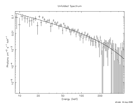
- Define the graphics interface before plotting the results of fitting the spectrum:
XSPEC12>cpd /Xw
XSPEC12>plot data res

XSPEC12>setplot energy
XSPEC12>plot uf |
Notes:
- cpd defines the graphics device; here xwindows.
- setplot changes the x-axis from channels to energy.
- plot indicates that the data and model should be plotted.
Spectra obtained for this example:
| Last updated by: Chuck Patterson 05/06/2011 |
|
|