Likelihood Tutorial: Binned
A step-by-step example of a binned likelihood analysis.
Prerequisites
- event data file (sometimes referred to as the photon data file or FT1 file)
- spacecraft data file
(also referred to as the pointing and livetime
history file or FT2 file)
See Extract LAT Data.
ScienceTools Popup Reference Window
Steps
1. Create a Counts Map
The examples in this web page were performed using a simulated data generated by gtobssim. The total simulation time was one day. Typically, one will want to create a counts map of the region-of-interest (ROI), summed over photon energies, in order to identify candidate sources and to ensure that the field looks sensible as a simple sanity check. For creating the counts map, we will use the gtbin application and select a 40 x 40 degree field containing the Crab, Geminga, and PKS 0528+134:
prompt> cat eventFiles galactic_back_events_0000.fits extragalactic_back_events_0000.fits ptsrcs_events_0000.fits prompt> gtbin This is gtbin version v2r0p3 Type of output file <CCUBE|CMAP|LC|PHA1|PHA2> [CMAP] : Event data file name [@eventFiles] : Output file name [Crab_cmap.fits] : Spacecraft data file name [../FT2/FT2.fits] : Size of the X axis in pixels [200] : 160 Size of the Y axis in pixels [200] : 160 Image scale (in degrees/pixel) [0.25] : Coordinate system (CEL - celestial, GAL -galactic) <CEL|GAL> [CEL] : First coordinate of image center in degrees (RA or galactic l) [83.57] : Second coordinate of image center in degrees (DEC or galactic b) [22.01] : Rotation angle of image axis, in degrees [0] : Projection method <AIT|ARC|CAR|GLS|MER|NCP|SIN|STG|TAN> [AIT] : STG prompt> |
The event data are contained in three files, extragalactic_back_events_0000.fits, galactic_back_events_0000.fits, and ptsrcs_events_0000.fits, so we have passed a text file containing those file names as the "Event data file".
NOTE: It is not appropriate to apply acceptance cone cuts on event data to be used for binned likelihood analysis, since the region-of-interest is defined as the boundaries of the counts map.
2. Identify Candidate Sources and Define the Source Model
The sources for Likelihood are defined using XML. The XML
document may be edited directly by hand, or the ModelEditor GUI may be used. For the purposes of this tutorial, we will include only the three strongest EGRET point sources in the anticenter region --- the Crab, Geminga, and PKS 0528+134 --- along with the interstellar and extragalactic diffuse components:
<?xml version="1.0" ?>
<source_library title="source library">
  <source name="Crab" type="PointSource">
    <spectrum type="PowerLaw2">
      <parameter free="1" max="1000.0" min="1e-05" name="Integral" scale="1e-06" value="15.4"/>
      <parameter free="1" max="0.0" min="-5.0" name="Index" scale="1.0" value="-2.19"/>
      <parameter free="0" max="200000.0" min="20.0" name="LowerLimit" scale="1.0" value="20.0"/>
      <parameter free="0" max="200000.0" min="20.0" name="UpperLimit" scale="1.0" value="200000.0"/>
    </spectrum>
    <spatialModel type="SkyDirFunction">
      <parameter free="0" max="360.0" min="-360.0" name="RA" scale="1.0" value="83.57"/>
      <parameter free="0" max="90.0" min="-90.0" name="DEC" scale="1.0" value="22.01"/>
    </spatialModel>
  </source>
  <source name="Geminga" type="PointSource">
    <spectrum type="PowerLaw2">
      <parameter free="1" max="1000.0" min="1e-05" name="Integral" scale="1e-06" value="10.2"/>
      <parameter free="1" max="0.0" min="-5.0" name="Index" scale="1.0" value="-1.66"/>
      <parameter free="0" max="200000.0" min="20.0" name="LowerLimit" scale="1.0" value="20.0"/>
      <parameter free="0" max="200000.0" min="20.0" name="UpperLimit" scale="1.0" value="200000.0"/>
    </spectrum>
    <spatialModel type="SkyDirFunction">
      <parameter free="0" max="360.0" min="-360.0" name="RA" scale="1.0" value="98.49"/>
      <parameter free="0" max="90.0" min="-90.0" name="DEC" scale="1.0" value="17.86"/>
    </spatialModel>
  </source>
  <source name="PKS 0528+134" type="PointSource">
    <spectrum type="PowerLaw2">
      <parameter free="1" max="1000.0" min="1e-05" name="Integral" scale="1e-06" value="9.802"/>
      <parameter free="1" max="0.0" min="-5.0" name="Index" scale="1.0" value="-2.46"/>
      <parameter free="0" max="200000.0" min="20.0" name="LowerLimit" scale="1.0" value="20.0"/>
      <parameter free="0" max="200000.0" min="20.0" name="UpperLimit" scale="1.0" value="200000.0"/>
    </spectrum>
    <spatialModel type="SkyDirFunction">
      <parameter free="0" max="360.0" min="-360.0" name="RA" scale="1.0" value="82.74"/>
      <parameter free="0" max="90.0" min="-90.0" name="DEC" scale="1.0" value="13.38"/>
    </spatialModel>
  </source>
  <source name="Galpro Diffuse" type="DiffuseSource">
    <spectrum type="ConstantValue">
      <parameter free="0" max="10.0" min="0.0" name="Value" scale="1.0" value="1.0"/>
    </spectrum>
    <spatialModel file="$(EXTFILESSYS)/galdiffuse/GP_gamma.fits" type="MapCubeFunction">
      <parameter free="0" max="1000.0" min="0.001" name="Normalization" scale="1.0" value="1.0"/>
    </spatialModel>
  </source>
  <source name="Extragalactic Diffuse" type="DiffuseSource">
    <spectrum type="PowerLaw">
      <parameter free="1" max="100.0" min="1e-05" name="Prefactor" scale="1e-07" value="1.6"/>
      <parameter free="0" max="-1.0" min="-3.5" name="Index" scale="1.0" value="-2.1"/>
      <parameter free="0" max="200.0" min="50.0" name="Scale" scale="1.0" value="100.0"/>
    </spectrum>
    <spatialModel type="ConstantValue">
      <parameter free="0" max="10.0" min="0.0" name="Value" scale="1.0" value="1.0"/>
    </spatialModel>
  </source>
</source_library>
|
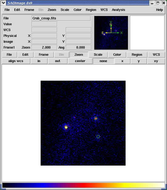
Here is the counts map of the Crab field with the three point sources indicated by the green circles:
3. Create a 3D Counts Map
For the likelihood analysis, a three-dimensional counts map with an energy axis is required. The gtbin aplication performs this tool with the CCUBE option. Since the spectra of gamma-ray sources are expected to be fairly featureless and modeled rather simply, 20 logarithmically spaced energy bands over the range 30 MeV to 200 GeV is sufficient:
prompt> gtbin This is gtbin version v2r0p3 Type of output file <CCUBE|CMAP|LC|PHA1|PHA2> [CMAP] : CCUBE Event data file name [@eventFiles] : Output file name [Crab_cmap.fits] : Crab_cmap_3D.fits Spacecraft data file name [../FT2/FT2.fits] : Size of the X axis in pixels [160] : Size of the Y axis in pixels [160] : Image scale (in degrees/pixel) [0.25] : Coordinate system (CEL - celestial, GAL -galactic) <CEL|GAL> [CEL] : First coordinate of image center in degrees (RA or galactic l) [83.57] : Second coordinate of image center in degrees (DEC or galactic b) [22.01] : Rotation angle of image axis, in degrees [0] : Projection method <AIT|ARC|CAR|GLS|MER|NCP|SIN|STG|TAN> [STG] : Algorithm for defining energy bins <FILE|LIN|LOG> [LOG] : Start value for first energy bin in MeV [20] : 30 Stop value for last energy bin in MeV [200000] : Number of logarithmically uniform energy bins [20] : prompt> |
4. Compute Livetimes
|
5. Compute Source Maps
These are model count maps of each source, i.e., multiplied by exposure and convolved with the effective PSF. The gtsrcmaps application performs this task:
prompt> gtsrcmaps Spacecraft data file [] : ../FT2/FT2.fits Exposure hypercube file [] : expCube.fits Counts map file [] : Crab_cmap_3D.fits Source model file [] : src_model.xml Binned exposure map [none] : Source maps output file [] : srcMaps.fits Response functions [HANDOFF] : Generating SourceMap for Crab....................! Generating SourceMap for Extragalactic DiffuseComputing binned exposure map....................! ....................! Generating SourceMap for GalProp Diffuse....................! Generating SourceMap for Geminga....................! Generating SourceMap for PKS 0528+134....................! prompt> |
If the binned exposure map file does not exist, then gtsrcmaps will compute an all-sky map with that name, using the energy bands of the 3D counts map. This exposure map can be reused for subsequent analyses of regions that cover the same time range and that use the same energy binning.
Since source map generation for the point sources is fairly quick, and maps for many point sources may take up a lot of disk space, it may be preferable to pre-compute the source maps for these sources at this stage. gtlike will compute these on the fly if they appear in the XML definition and a corresponding map is not in the source maps FITS file. To skip generating source maps for point sources, specify "ptsrc=no" on the command line when running gtsrcmaps.
6. Run gtlike
Now we are ready to run the gtlike application:
prompt> gtlike sfile=anticenter_fit.xml Statistic to use (BINNED|UNBINNED) [BINNED] Counts map file[srcMaps.fits] Binned exposure map[none] Exposure hypercube file[expCube.fits] Source model file[src_model.xml] Response functions to use[HANDOFF] Optimizer (DRMNFB|NEWMINUIT|MINUIT|DRMNGB|LBFGS) [MINUIT] <...skip some output...> Crab: Integral: 21.7136 +/- 4.14233 Index: -2.27117 +/- 0.0884106 LowerLimit: 20 UpperLimit: 200000 TS value: 361.223 Extragalactic Diffuse: Prefactor: 1.76209 +/- 0.145828 Index: -2.1 Scale: 100 GalProp Diffuse: Value: 1 Geminga: Integral: 12.2414 +/- 1.46925 Index: -1.7131 +/- 0.0438393 LowerLimit: 20 UpperLimit: 200000 TS value: 1424.71 PKS 0528+134: Integral: 6.35981 +/- 3.34248 Index: -2.3426 +/- 0.234661 LowerLimit: 20 UpperLimit: 200000 TS value: 37.4594 WARNING: Fit may be bad in range [30, 46.5926] (MeV) WARNING: Fit may be bad in range [34375.4, 53388] (MeV) Total number of observed counts: 2389 Total number of model events: 2452.06 -log(Likelihood): 12664.63356 Writing fitted model to anticenter_fit.xml Elapsed CPU time: 18.35 prompt> |
Note that we have passed the command line option "sfile=anticenter_fit.xml" so that the results are saved in an XML file, which we will use for creating a model counts map based on this fit.
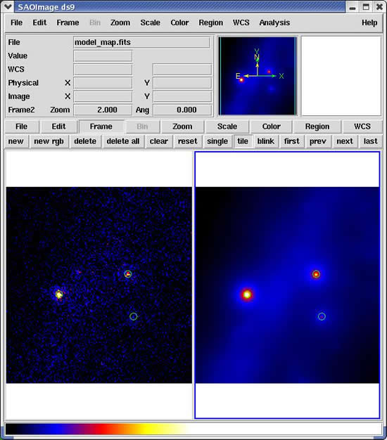
7. Create a Model Map
For comparison to the counts map data, we create a model map of the region based on the fit parameters. This map is essentially an infinite-statistics counts map of the region-of-interest based on our model fit.The gtmodel application reads in the fitted model, applies the proper scaling to the source maps, and adds them together to get the final map.
prompt>gtmodel Source maps file [srcMaps.fits] : Source model file [srcModel.xml] : src_model.xml Output file [model_map.fits] : Response functions [HANDOFF] : prompt> |
The following shows the energy-summed counts map and the corresponding model map.
Related FTOOLS
Owned by: Jim Chiang
Generated on: Wed Apr 6 07:50:21 2005
Last update generated by Analia Cillis: 03/14/2008
| Last updated by: Analia Cillis and Chuck Patterson 03/14/2008 |