CALRECON 2005/03/09

---

• I work on the direction and energy reconstruction above 5 GeV (5 to 50 GeV, 0 to 60°);
• Nothing new on the direction reconstruction;
• Updated results on energy reconstruction.
  • Using the two profile fits I've already shown;
  • Trying to improve the profile fit : using a "propagator" like tool.

---

USING THE TWO PROFILE FITS

Before fitting:

• retrieving the trajectory information (from tracker, from calo if no track)
• considering the gamma as a cylinder with a radius = 20mm (Moliere radius = 35mm)
• determining the intersection of that cylinder with each tower and each layer
• converting the layers boundaries in X0 units

The two profile fits:

• my "standard" average profile (2 parameters);
• "my" profile (not average one) (3 parameters).

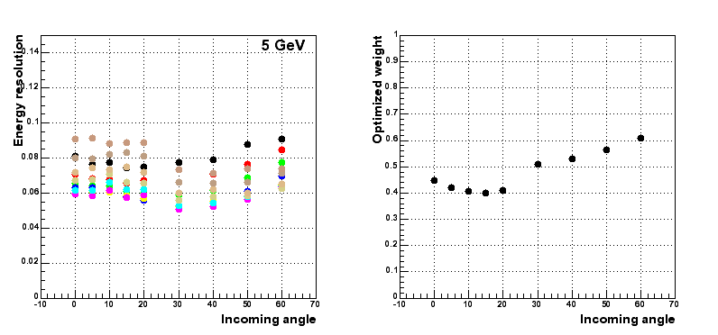
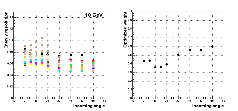
The tendency was that the average profile was better below theta = ~40°, and above ~40° my profile was slightly better.

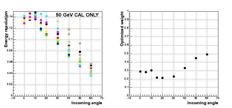
So one can check if it is possible to optimize the resolution by taking the weighted average of the two profiles :
E = p * Emyprof + (1-p) * Eprofaverage

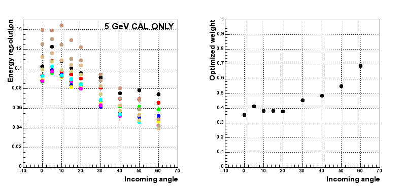
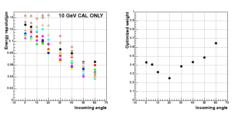
For each weight between 0 and 1, I plot the resolution as function of the incoming angle. For each incoming angle, I determine which weight optimizes the resolution.

---

Results for events with tracker information :

---

Results for CAL ONLY events : worse than for events with a track since the shower is in average less contained.

---

TRYING TO IMPROVE THE PROFILE FIT : USING A "PROPAGATOR" LIKE TOOL

The triggering idea : at large incoming angle, the deposited energy in a slice of the shower perpendicular to the shower axis is shared between two or more layers. This is not taken into account in my previous profile fits (I only converted the layers boundaries in X0 units).

In order to quantify this effect I have implemented a kind of propagator:

• moving along the shower trajectory in millimeters;
• at each step :
  • considering a disk of thickness dz millimeters and radius r;
  • determining what fraction of disk of thickness dz millimeters and radius r is in the CsI, in the crack and out of glast;
  • determining the effective radiation length seen by the disk;
  • converting the position of the disk from millimeters to X0 units;
  • determining the fraction of the disk which is in the layer number i (layer mixing effect);

The profile fit can use these layer fractions along the shower trajectory to predict the energies in the layers.

---

THE OBVIOUS QUESTION AT THIS STAGE IS : WHAT RADIUS SHOULD WE USE ?

In Bill Atwood's talk (dec 2002), he suggests to consider :

• a core : r ~ Moliere radius = 35 mm in CsI;
• a fringe : 2 * Moliere radius.

The Moliere radius = 35 mm, which is big compared to the height of a layer = 21.35 mm => the layer mixing effect is very large !

I have used the resuts from G. GRINDHAMMER and S. PETERS (The parameterized simulation of electromagnetic showers in homogeneous and sampling calorimeters - Presented at International Conference on Monte Carlo Simulation in High-Energy and Nuclear Physics - MC 93, Tallahassee, Florida, 22-26 Feb 1993) in order to derive an effective Moliere radius as function of the position in the shower.

To describe the average radial energy profile, Grindhammer and Peters use the following function:
f(r) = p * f_core(r) + (1-p) * f_tail(r) with f_core and f_tail having the same form : 2 r R² / (r² + R²)²

So we describe the average radial enerfy profile with three parameters : Rcore, Rtail and p.
In their paper they give the functions of Rcore, Rtail and p as function of the position in the shower t / Tmax (Tmax is the position of the maximum of the shower).

We can determine how the radius containing 68% (or 90%) of the energy varies with the position in the shower.


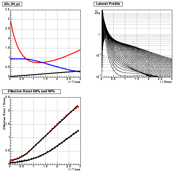
This result shows that before the maximum of the shower, the effective radius is much smaller than the Moliere radius. But it is clear that choosing R(90%) instead of R(68%) will increase very much the layer mixing effect.

---

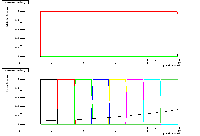
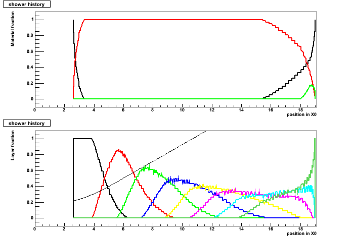
ILLUSTRATING THE LAYER MIXING EFFECT

One event at theta = 0° : (no layer mixing)

Upper plot = material fraction :

• black : outside Glast;
• red : inside CsI;
• green : inside cracks;

Bottom plot = layer fraction : (the function is R(68%) as function of the position in the shower)

• black : layer 0
• red : layer 1
• ...

---

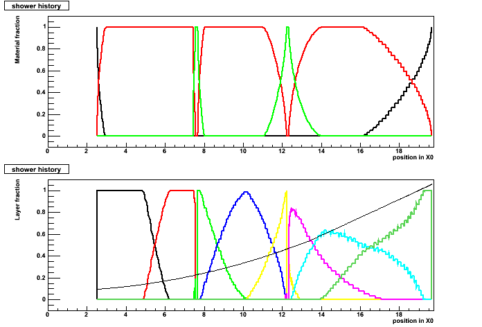
One event at theta = 60° :

Using R(68%)


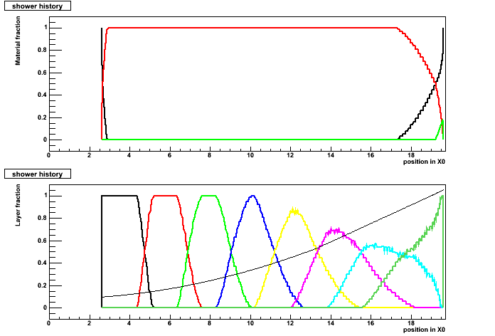
Using R(90%)

---

One event with a complex history at theta = 60° (2 cracks):

---

The first results (very preliminary) about the energy resolution using this layer fractions correction are not better than with the "naive" profiles...

NEXT STEP : instead of using R(xx%), use directly the function f(r).