LAT and GBM Joint Spectral Analysis
This procedure provides all information needed to do the joint analysis with GBM (BGO and NaI) and LAT data.
Notes: Xspec is used as a spectral analysis tool in this procedure because it can handle multiple
data sets and response matrices for the same spectral model, making joint analysis of GBM and LAT data possible.
The current version of Xspec works on Windows under Cygwin.
Prerequisites
- ScienceTools v6r0p5, or later
- dataSubselector v3r6, or later
Notes:
- Data files were obtained with observationSim, and the sky model includes:
- The extra galactic diffuse emission
- The GRB under study is the GRB simulated with the GRBobs model
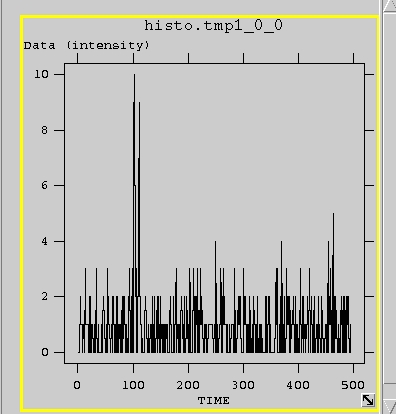
- A few hundreds seconds (500) of simulated sky with observationSim (v5r8p3 ) were run, and the resulting FITS files are:
If you plot the "TIME" column of the first file you will find something like this, showing the LAT event data with the simulated bursts at 100 s.
The simulation produces also the following files which are needed by the GBM simulators:
Note: These files are not needed for the analysis !!! The GBM team will take these files and produce the GBM output FITS file.
The GBM output files which you will need are located at:
http://www.slac.stanford.edu/exp/glast/workbook/sciToolsData/
latGbmJtSpectralAnal/GBM_BN050718001
You are now ready to start the analysis.
Steps:
- Select LAT data
- Bin the LAT data
- Bin the GBM data
- Compute the response matrix for the LAT
- Use XSPEC for spectral analysis
- LAT binned spectral analysis
- Combined GBM+LAT spectral fit
1) Extract the LAT data (dataSubselector)
Go to dataSubselector executable directory, and:
[omodei@pcglast35 rh9_gcc32]$ ./gtselect.exe
Input FT1 file [...] :/data1/glast/GRBdata/test_events_0000.fits
Output FT1 file [...] : /data1/glast/GRBdata/GRB_050718001_LAT.fits
RA for new search center (degrees) <0 - 360> [...] : 23.8
Dec for new search center (degrees) <-90 - 90> [...] : -14.2
radius of new search region (degrees) <0 - 180> [...] : 20
start time (MET in s) [...] : 100
end time (MET in s) [...] : 150
lower energy limit (MeV) [...] : 30
upper energy limit (MeV) [...] : 200000
first conversion layer <0 - 15> [0] :
last conversion layer <0 - 15> [15] :
Done. |
This will produce the FITS file: GRB_050718001_LAT.fits
Notice that the procedure requires the "true" Ra and the Dec and the starting time of the GRB. You can use fv to inspect the original "LAT events" file for estimating them.
2) Binning the LAT extracted data (evtbin)
Go to the evrbin executable dir and:
[omodei@pcglast35 rh9_gcc32]$ ./gtbin.exe
gtbin: INFO: This is gtbin version v0r10p1
Type of output file <CMAP|LC|PHA1|PHA2> [PHA1] :
Event data file name [...] : /data1/glast/GRBdata/GRB_050718001_LAT.fits
Output file name [...] : /data1/glast/GRBdata/GRB_050718001_LAT.pha
Spacecraft data file name [...] : /data1/glast/GRBdata/test_scData_0000.fits
Algorithm for defining energy bins <FILE|LIN|LOG> [LOG] :
Start value for first energy bin [30] :
Stop value for last energy bin [200000] :
Number of logarithmically uniform energy bins [15] : |
This will produce the PHA1 FITS file: GRB_050718001_LAT.pha
3) Binning the GBM data (evtbin)
Let's start with the BGO 1 detector (label B1):
[omodei@pcglast35 rh9_gcc32]$ ./gtbin.exe
gtbin: INFO: This is gtbin version v0r10p1
Type of output file <CMAP|LC|PHA1|PHA2> [PHA1] :
Event data file name [...] : /data1/glast/GRBdata/GBM_BN050718001/GLG_TTE_B1_BN050718001_V01.fits
Output file name [...] : /data1/glast/GRBdata/GRB_050718001_B1.pha
Spacecraft data file name [...] : NONE |
And then let's compute the NaI 6 detector (which is the one with more counts):
[omodei@pcglast35 rh9_gcc32]$ ./gtbin.exe
gtbin: INFO: This is gtbin version v0r10p1
Type of output file <CMAP|LC|PHA1|PHA2> [PHA1] :
Event data file name [...] : /data1/glast/GRBdata/GBM_BN050718001/GLG_TTE_N6_BN050718001_V01.fits
Output file name [...] : /data1/glast/GRBdata/GRB_050718001_N6.pha
Spacecraft data file name [NONE] : |
Now you have also GRB_050718001_B1.pha and GRB_050718001_N6.pha PHA1 file.
Notice that the new evtbin allows NONE as spacecraft data!
4) Compute the response matrix for the LAT data (rspgen)
[omodei@pcglast35 rh9_gcc32]$ ./gtrspgen.exe
gtrspgen: INFO: This is gtrspgen version v0r6p0
Response calculation method (GRB, PS) <GRB|PS> [GRB] :
Spectrum file name [/data1/glast/GRBdata/GRB_050718001_LAT.pha] :
Spacecraft data file name [/data1/glast/GRBdata/test_scData_0000.fits] :
Output file name [/data1/glast/GRBdata/GRB_050718001_LAT.rsp] :
True RA of point source (degrees) [23.8] :
True DEC of point source (degrees) [-14.2] :
Time of GRB (s) [100] :
Radius of circle for PSF integration (degrees) [20] :
Response function to use, e.g. DC1F/DC1B, G25F/G25B, TestF/TestB [TestF] :
Algorithm for defining true energy bins <FILE|LIN|LOG> [LOG] :
Start value for first energy bin [15] : 30
Stop value for last energy bin [3000000] : 200000
Number of logarithmically uniform energy bins [100] : 15 |
Using XSPEC for spectral analysis
You now have all the files needed to perform a spectral analysis using xspec. These include:
| GBM BGO (B1) data file |
GRB_050718001_B1.pha |
| GBM NaI (N6) data file |
GRB_050718001_N6.pha |
| LAT data file |
GRB_050718001_LAT.pha |
| GBM BGO (B1) Detector Response Matrix (DRM) |
GLG_CSPEC_B1_BN050718001_V01.RSP |
| GBM NaI (N6) DRM |
GLG_CSPEC_N6_BN050718001_V01.RSP |
| LAT DRM |
GRB_050718001_LAT.rsp |
| GBM BGO (B1) Background |
GLG_BCK_B1_BN050718001_V01.BAK |
| GBM NaI (N6) Background |
GLG_BCK_N6_BN050718001_V01.BAK |
Notice that the LAT does not have any background file since it has a negligible background !
a) Spectral Binned analysis for LAT data:
fitting the high energy component with a power law model
Another test that can be easily done is the LAT only spectral analysis, fitting the High Energy part of the GRB050718001 spectrum with a power law.
This is the xspec sequence of commands:
[omodei@pcglast35 GRBdata]$ xspec11
Xspec 11.3.2 15:14:15 14-Jul-2005
For documentation, notes, and fixes see http://xspec.gsfc.nasa.gov/
Plot device not set, use "cpd" to set it
Type "help" or "?" for further information
XSPEC>cpd /xw
XSPEC>data GRB_050718001_LAT.pha
Net count rate (cts/s) for file 1 0.8000 +/- 0.1265
1 data set is in use
XSPEC>resp GRB_050718001_LAT.rsp
XSPEC>setplot energy
XSPEC>plot ldata
XSPEC>mod po
Model: powerlaw<1>
Input parameter value, delta, min, bot, top, and max values for ...
1 0.01 -3 -2 9 10
1:powerlaw:PhoIndex>
1 0.01 0 0 1E+24 1E+24
2:powerlaw:norm>
---------------------------------------------------------------------------
---------------------------------------------------------------------------
Model: powerlaw<1>
Model Fit Model Component Parameter Unit Value
par par comp
1 1 1 powerlaw PhoIndex 1.00000 +/- 0.00000
2 2 1 powerlaw norm 1.00000 +/- 0.00000
---------------------------------------------------------------------------
---------------------------------------------------------------------------
Chi-Squared = 2.4111920E+11 using 15 PHA bins.
Reduced chi-squared = 1.8547630E+10 for 13 degrees of freedom
Null hypothesis probability = 0.00
XSPEC>fit
---------------------------------------------------------------------------
Variances and Principal axes :
1 2
1.99E-04 | -1.00 0.00
4.72E+04 | 0.00 -1.00
---------------------------------------------------------------------------
---------------------------------------------------------------------------
Model: powerlaw<1>
Model Fit Model Component Parameter Unit Value
par par comp
1 1 1 powerlaw PhoIndex 2.18267 +/- 0.195939
2 2 1 powerlaw norm 110.575 +/- 217.335
---------------------------------------------------------------------------
---------------------------------------------------------------------------
Chi-Squared = 3.152037 using 15 PHA bins.
Reduced chi-squared = 0.2424644 for 13 degrees of freedom
Null hypothesis probability = 0.997
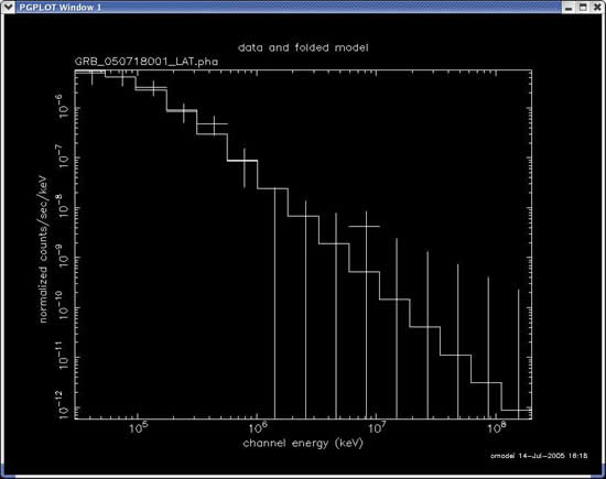
XSPEC>plot ldata |
Notice that the power law index is in agreemant with the input value 2.25, with a good chi square!
b) LAT and GBM joint spectral fitting: the first GRB viewed in 6 decades of energy !
Start xspec, and set the plot device to x-window:
[omodei@pcglast35 GRBdata]$ xspec11
Xspec 11.3.2 15:14:15 14-Jul-2005
For documentation, notes, and fixes see http://xspec.gsfc.nasa.gov/
Plot device not set, use "cpd" to set it
Type "help" or "?" for further information
XSPEC>cpd /xw |
Load the data...
XSPEC>data GRB_050718001_B1.pha GRB_050718001_N6.pha GRB_050718001_LAT.pha
Net count rate (cts/s) for file 1 953.2 +/- 5.942
Net count rate (cts/s) for file 2 479.5 +/- 4.215
Net count rate (cts/s) for file 3 0.8000 +/- 0.1265
3 data sets are in use |
...the responses...
| XSPEC>resp GBM_BN050718001/GLG_CSPEC_B1_BN050718001_V01.RSP GBM_BN050718001/GLG_CSPEC_N6_BN050718001_V01.RSP GRB_050718001_LAT.rsp |
... and the backgrounds for the 2 GBM detectors:
XSPEC>back GBM_BN050718001/GLG_BCK_B1_BN050718001_V01.BAK GBM_BN050718001/GLG_BCK_N6_BN050718001_V01.BAK
*WARNING*: Data and background channel type
(PI,PHA) for file 1
*WARNING*: Data and background channel type
(PI,PHA) for file 2
Net count rate (cts/s) for file 1 235.2 +/- 8.955 ( 24.7% total)
using response (RMF) file... GBM_BN050718001/GLG_CSPEC_B1_BN050718001_V01.RSP
using background file... GBM_BN050718001/GLG_BCK_B1_BN050718001_V01.BAK
Net count rate (cts/s) for file 2 255.1 +/- 5.639 ( 53.2% total)
using response (RMF) file... GBM_BN050718001/GLG_CSPEC_N6_BN050718001_V01.RSP
using background file... GBM_BN050718001/GLG_BCK_N6_BN050718001_V01.BAK |
Now you can plot the raw data (counts vs channels):
The results should be the following:
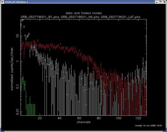
The color code is:
White: BGO data (B1)
Red: NaI data (N6)
Green: LAT data (LAT)
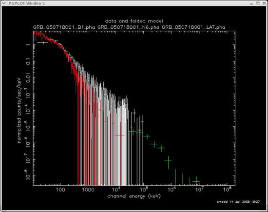
Set the x-axis in energy instead of channels:
XSPEC>setplot energy
XSPEC>plot ldata |
Suggestion from Valerie Connaughton: BGO detector's effective area starts from 30 keV, but we now that the BGO operational mode is such that it electronically works at gains that enhance the high energy counts, at the expense of the low energy counts (measured by the NaI detector). Counts below ~150 keV should be thrown away. (first dataset)
Vice versa, we should throw out the NaI counts above 1MeV. (second dataset)
XSPEC>ignore 1:**-150.
ignoring channels 1 - 8 in dataset 1
XSPEC>ignore 2:1000.-**
ignoring channels 107 - 128 in dataset 2
XSPEC>plot ldata |
This is the result:

Now you can load the 4 parameters 'Band' model (grbm):
XSPEC>mod grbm
Model: grbm<1>
Input parameter value, delta, min, bot, top, and max values for ...
-1 0.01 -10 -3 2 5
1:grbm:alpha>
-2 0.01 -10 -5 2 10
2:grbm:beta>
300 10 10 50 1E+03 1E+04
3:grbm:tem>
1 0.01 0 0 1E+24 1E+24
4:grbm:norm>
---------------------------------------------------------------------------
---------------------------------------------------------------------------
Model: grbm<1>
Model Fit Model Component Parameter Unit Value
par par comp
1 1 1 grbm alpha -1.00000 +/- 0.00000
2 2 1 grbm beta -2.00000 +/- 0.00000
3 3 1 grbm tem keV 300.000 +/- 0.00000
4 4 1 grbm norm 1.00000 +/- 0.00000
---------------------------------------------------------------------------
---------------------------------------------------------------------------
Chi-Squared = 7.3980832E+07 using 241 PHA bins.
Reduced chi-squared = 312155.4 for 237 degrees of freedom
Null hypothesis probability = 0.00
XSPEC>fit
Chi-Squared Lvl Fit param # 1 2 3 4
684.699 -3 -0.3483 -2.105 125.7 1.6080E-02
172.148 -4 -0.5064 -2.163 100.2 1.8108E-02
141.504 -5 -0.3491 -2.232 81.88 2.2567E-02
136.551 -6 -0.3566 -2.258 84.29 2.2764E-02
136.541 -7 -0.3571 -2.259 84.23 2.2745E-02
136.541 -8 -0.3571 -2.259 84.24 2.2747E-02
---------------------------------------------------------------------------
Variances and Principal axes :
1 2 3 4
2.26E-07 | -0.01 0.00 0.00 1.00
5.10E-04 | 0.47 0.88 0.01 0.00
9.63E-04 | -0.88 0.47 -0.01 -0.01
7.07E+01 | 0.01 0.00 -1.00 0.00
---------------------------------------------------------------------------
---------------------------------------------------------------------------
Model: grbm<1>
Model Fit Model Component Parameter Unit Value
par par comp
1 1 1 grbm alpha -0.357092 +/- 0.957403E-01
2 2 1 grbm beta -2.25877 +/- 0.256844E-01
3 3 1 grbm tem keV 84.2376 +/- 8.40691
4 4 1 grbm norm 2.274691E-02 +/- 0.351060E-02
---------------------------------------------------------------------------
---------------------------------------------------------------------------
Chi-Squared = 136.5413 using 241 PHA bins.
Reduced chi-squared = 0.5761235 for 237 degrees of freedom
Null hypothesis probability = 1.00
XSPEC>plot ldata |
The high energy power law perfectly agree with the input parameter, and the reduced chi square is very good indicating the goodness of fit, and that the effect of the GBM data in constraining the parameters of the model.
The graphical output is the following:
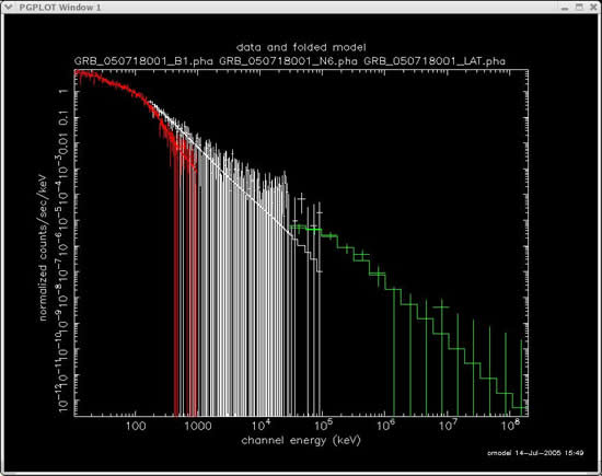
Important!!
For the non x-spec users (like myself) the way to plot the results of xspec can be not obvious!
The data (dot with error bars) are NOT normalized by the effective area of the detectors, so that they represents the "raw counts" (divided by the exposure and by the energy bin width.
The model (in this case the Band function) is represented "folded" with the DRM. This means that in the above plot, the curve is ONLY ONE MODEL, as seen by different detectors. There is no reason to expect a continuity between one detector and the other. The only thing the observer should care is how well the data lie on the fit and how good is the chi-square (or other goodness estimators)!
| |
True |
Reconstructed (XSPEC) |
| Low Energy spectral index (alpha) |
-0.4 |
-0.36 +/- 0.1 |
| High Energy Spectral index (beta) |
-2.25 |
-2.26 +/- 0.03 |
| E0 |
~90 keV |
84.2376 +/- 8.4069 keV |
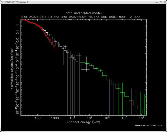
For plotting purposes, you can choos to rebin the data, setting the minimum significance (in sigma) and the maximum number of bins which will be merged. My choice was to rebin only BGO and NaI data:
XSPEC>setplot rebin 5 8 1
XSPEC>setplot rebin 5 5 2
XSPEC>plot ldata |
to produce this output:
| Last updated by: Analia Cillis
02/27/2008 |
|
|