In this thread we will look at a map of the photons in the region around a source, and at a lightcurve of the photons from a source. To make the example concrete, we will investigate a suspected burst.

SciTools Reference Pages: If you want the SciTools Reference pages to open in a popup window, click on: Open Popup Reference Window.

Prerequisites

It is assumed that:

• The GBM reported that a burst occurred at:

• RA = 45.2867
• Dec = -9.83695
• Tstart = 254033757. s (Mission Elapsed Time)
• Duration = ~ 6 s

• You have downloaded the files used in this tutorial from:

http://www.slac.stanford.edu/exp/glast/workbook/sciToolsData/
exploreLatData/LAT_explore.tgz

These files include:

• grb_ft1.fits
• GRB090119205_lc.fits
• GRB090119205_lc_ft1.fits
• GRB090119205_lc.png
• GRB090119205_map.fits
• GRB090119205_map_ft1.fits
• GRB090119205_map.png

Steps

The analysis steps are:

1. Extract the Data

2. Data Selections

3. Bin the Data

4. Look at the Data

Note: The grb_ft1.fits file used in this tutorial is included in the zip file downloaded earlier. (Refer to Prerequisites.)

For instructions on obtaining new data, refer to: Extract LAT Data.

To map out the region of the burst, you want a large region from a short time range, while for the lightcurve you want a small region around the burst from a long time range. You will therefore need to make two different selections:

Start up gtselect.

Note: For this example the photon file downloaded from the GSSC website has been renamed grb_ft1.fits.

The following is a transcript of running this tool:

glitch [168] [cillis]: gtselect
Input FT1 file [grb_ft1.fits] : 
Output FT1 file [GRB090119205_map_ft1.fits] : 
RA for new search center (degrees) <0 - 360> [45.2867] : 
Dec for new search center (degrees) <-90 - 90> [-9.83695] : 
radius of new search region (degrees) <0 - 180> [35] : 
start time (MET in s) [254033707] : 
end time (MET in s) [254034457] : 
lower energy limit (MeV) [30] : 
upper energy limit (MeV) [200000] : 
Event classes (-1=all, 0=Front, 1=Back) <-1 - 4> [-1] : 
Done.
glitch [169] [cillis]: 
            

Notes:

• The input photon file is grb_ft1.fits, and the output file is GRB090111402_map_ft1.fits.

• A circular region with radius 35 degree around the burst location from a 700 s time period has been selected, and an energy cut has been made (i.e., only photons between 30 MeV and 200 GeV are selected).

• The '-1' under Event classes indicates that the broadest class of photons will be used.

Run the tool again, this time with a smaller region but a longer time range. Currently the time ranges for both the photon map and the lightcurve are the same. In creating this analysis thread, we actually plotted the map before running gtselect, and we found that the LAT photons are centered on RA=47.907, Dec=-11.758.

(Since gtselect is an FTOOL, it uses as defaults the values from the previous run, not the parameter values used to create the input photon file.)

glitch [170] [cillis]: gtselect
Input FT1 file [grb_ft1.fits] : 
Output FT1 file [GRB090119205_map_ft1.fits] : GRB090119205_lc_ft1.fits
RA for new search center (degrees) <0 - 360> [45.2867] : 47.907
Dec for new search center (degrees) <-90 - 90> [-9.83695] : -11.758
radius of new search region (degrees) <0 - 180> [35] : 10
start time (MET in s) [254033707] : 
end time (MET in s) [254034457] : 
lower energy limit (MeV) [30] : 
upper energy limit (MeV) [200000] : 
Event classes (-1=all, 0=Front, 1=Back) <-1 - 4> [-1] : 
Done.
glitch [171] [cillis]:
            

Notes:

• A new output file has been provided.
• The search radius is reduced to 10 degrees.
• The start to stop time range has been expanded.
• The center of the region has been moved.

Use gtbin to bin the photon data into a photon map and a lightcurve.

First create the photon map. The following is the transcript of running this tool:

glitch [173] [cillis]: gtbin
This is gtbin version v2r0p3
Type of output file <CCUBE|CMAP|LC|PHA1|PHA2> [CMAP] : 
Event data file name [GRB090119205_map_ft1.fits] : 
Output file name [GRB090119205_map.fits] : 
Spacecraft data file name [FT2.fits] : 
Size of the X axis in pixels [50] : 
Size of the Y axis in pixels [50] : 
Image scale (in degrees/pixel) [0.5] : 
Coordinate system (CEL - celestial, GAL -galactic) <CEL|GAL> [CEL] : 
First coordinate of image center in degrees (RA or galactic l) [47.907] : 
Second coordinate of image center in degrees (DEC or galactic b) [-11.758] : 
Rotation angle of image axis, in degrees [0] : 
Projection method <AIT|ARC|CAR|GLS|MER|NCP|SIN|STG|TAN> [AIT] : 
glitch [174] [cillis]: 
            

Notes:

• Select cmap (i.e., count map) as the output.

• When we ran gtselect we called the file from a large area GRB0090119205_map_ft1.fits.

• The count map file will be called GRB090119205_map.fits.

• The spacecraft data file that we extracted is FT2.fits.

• Although in gtselect we selected a circular region with a 35 degree radius, we will form a count map with 50 pixels in each direction, with each pixel 1/2 degree on a side.

• Even though in gtselect we selected a region centered on the GBM burst location, we enter the center of the region to be mapped as the coordinates found for LAT photons: RA=47.907, DEC=-11.758.

Now, we create the lightcurve. The following is the transcript of running this tool.

glitch [183] [cillis]: gtbin
This is gtbin version v2r0p3
Type of output file <CCUBE|CMAP|LC|PHA1|PHA2> [LC] : 
Event data file name [GRB090119205_lc_ft1.fits] : 
Output file name [GRB090119205_lc.fits] : 
Spacecraft data file name [FT2.fits] : 
Algorithm for defining time bins <FILE|LIN|SNR> [LIN] : 
Start value for first time bin in MET [254033707] : 
Stop value for last time bin in MET [254034457] : 
Width of linearly uniform time bins in MET [10] : 
glitch [184] [cillis]: 
            

Notes:

• gtselect was used to create GRB0090119205_lc_ft1.fits, a photon list from a small region but a long time range.

• gtbin will bin these photons and output the result into GRB090119205_lc.fits.

There are a number of options for choosing the time bins. Here we have chosen linear bins with equal time widths of 10 seconds.

We now have two FITS files with binned data; one with a lightcurve (GRB090119205_lc.fits), and a second with a count map (GRB090119205_map.fits).

Note: Currently we do not have any GLAST specific graphics programs, but there are many tools available to plot data in FITS files, such as fv and ds9. Here we use fv.

To look at the count map:

1. First start up fv.

2. Then open GRB090119205_map.fits. Click on 'open file' to get the 'File Dialog' GUI. Choose 'GRB090119205_map.fits'. A new GUI will open up with a table with two rows.

3. FITS files consist of a series of extensions with data. Since the count map is an image, it is stored in the primary(=first) extension (for historical reasons only images can be stored in the primary extension). Clicking on the 'Image' button in the first row results in:

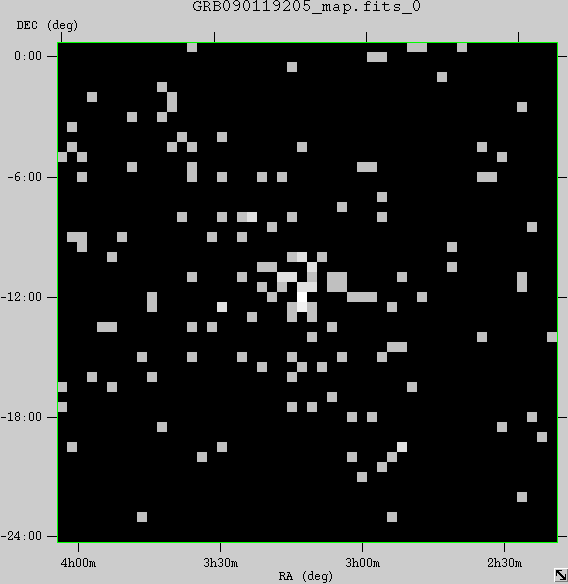
Observe that there are many pixels with a few counts each near the burst location, and few pixels with any counts away from the burst.

To look at the lightcurve:

1. Open burst_lightcurve.fits. Start up fv. Choose the file 'GRB090119205_lc.fits' in the File Dialog GUI.

The extension GUI has three rows since there are three extensions. Since the lightcurve is in the RATE extension, choose 'all' in the second row. The extension has 3 columns: TIME, TIMEDEL and COUNTS.

The time bins were created to have a width of 10 s, and therefore TIMEDEL is always 10.

2. Now plot the COUNTS as a function of TIME. Select 'plot' from the 'tools' drop-down menu in the extension GUI. Click on 'Time' then on 'x'. Click on 'Counts' then on 'y'. Finally click on 'Go'. The result is:

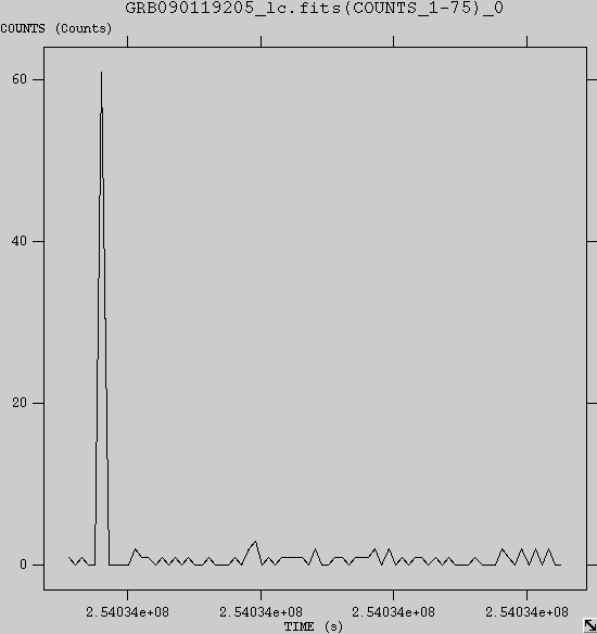
Note: Except for the burst, almost all bins have 0 counts, with only an occasional bin with one count. This demonstrates that there is essentially no background for LAT observations of gamma-ray bursts.