LAT Software Overview: ACD, TKR, and CAL
Start with:
- LAT-Rochester-1 ;p10-on really great; p8-9 useful; earlier pages may be of help.
- LAT Data Analysis Primer, March 8,2005 p40-
- Also see: Best_Sources PNGs
The LAT identifies and measures the flux of cosmic Gamma-rays with energies from ~10 MeV to ~300 GeV. The Gamma-rays pass undetected through the ACD, convert to electron-positron pairs in the tracker, and deposit their energies in the calorimeter. The instrument triggers when a track segment traverses any three contiguous silicon layers, which are composed of two silicon planes, each measuring one direction perpendicular to the tower axis.
Photons are detected as discrete "events", consisting of the tracks (energy deposit) left by ionizing particles in different parts of the instrument. These events need to be classified as incident charged particles or photon-induced particle pairs. The ability to separate charged particles from gamma-ray pair events determines the level of background contaminating the sample.
Key LAT Components
Hardware:- ACD – Segmented Anticoincidence Detector:
- 89 plactic scintillator tiles
- Rejects background of charged cosmic rays.
- TKR – Precision Si-strip Tracker:
- 18 XY tracking layers with tungsten foil converters.
- Single-sided silicon strip detectors (228 μm pitch, 900k strips)
Note: Segmentation mitigates self-veto effects at high energy.
- Measures photon direction.
- Gamma ID.
- CAL – Hodoscopic CsI Calorimiter:
TKR information is used to precisely identify the impact point and the path length of the ions in the plastic scintillators of the ACD and the CsI logs of the CAL.
- Array of 1536 CsI(Tl) crystals in 8 layers [mounted beneath each of the 16 TKR towers (12 crystals in each of 8 layers X 16 towers = 1536 crystals total).
- Measures the photon energy.
- Images the shower.
Electronics System:
- Electronics system includes:
- Flexible, robust hardware trigger.
- Software filters.
Note: Heavy ion events are collected in parallel to photons for science data, thanks to a flexible trigger logic that is able to select different type of events and activate specific readout modes. Heavy ions are triggered by a special high level discriminator in the ACD and followed to the CAL using TKR information.
Background Flux: ???
Geometry detail includes:
- Tracker electronics boards
- Mounting holes in ACD tiles
- Spacecraft details
- ...
Note: Over 45,000 (???) volumes and growing (as of Feb 2, 2007); see: ???
Background Flux Calculation
Note to self: LAT-Rochester-1.pdf pp. 4-5; Also see Background Flux Review - J. ormes et al., LAT-TD-08316-01:
- Albedo e+e- flux a factor >3 larger than for PDR ???
- Primary cosmic proton flux is higher ???
- New Albedo g flux ???
- Variations over one day (see Update of Albedo g spectrum, Petry, D., 2005, AIP Conf Proc. 745, 709-714, astro-ph/041087
- galactic CR protons
- He+CNO
- galactic CR e+e-
- albedo (reentrant+splashback) p+pbar
- albedo (reentrant+splashbac) e+e-
- albedo gamma
Plus: simulation of Sout Atlantic Anomaly, satellite rocking
Simulation (Based on GEANT4)
See: LAT-Rochester-1.pdf pp 6;
Interaction Physics: ???
- QED (???) - derived from GEANT3 with extensions to higher and lower energies (alternate models available) ???
- Hadronic - based on GEISHA (alternate models available) ???
Propagation:
- Full treatment of multiple scattering (MS); see ???
- Medium-dependent range cut-off ???
- Surface-to-surface ray tracing ???
Information from actual LAT tests:
- Detailed instrument response
- Dead Channels
- Noise
- etc. ???
Overall Deadtime Effects: ???
Instrument Response:
- Energy deposit given by GEANT is turned into the signals that would be recorded in the detectors.
- Tracker:
- Tower Triggers.
- Hits strips when energy is above threshold.
- Time-over-threshold ORs with correct gains.
- Calorimeter:
- Correct sharing of signal between two ends of crystals (attenuation).
- Signals in small and large diodes, each with two ranges.
- Anticoincidence Detector
- Signals from tiles to both phototubes.
- Correct sharing of signals between two ends of ribbons (attenuation).
- Tracker:
Instrument Triggering and Onboard Data Flow:
Hardware Trigger. The hardware trigger, based on prescribed combinations of special signals from each tower, initiates readout.
Function:
- Did anything happen? reword
- Keep as simple as possible. ???
Combinations of trigger primitives:
- TKR - 3 x•y pair layers in a row
- CAL:
- LO - independent check, energy info.
- HI - indicates high energy event.
Note: Instrument Total Rate: <3 kHz>, using ACD veto in hardware trigger. ???
When a trigger occurs, all subsystems are read out in ~27 μs
Onboard Processing:
- Onboard filters:
- Reduce data to fit within downlink.
- Provide samples for systematic studies.
- Flexible, loose cuts.
- Actual FSW filter code is wrapped and embedded in teh full detector simulation
- Signal/background can be tuned:
- g rate: a few Hz
- Total downlink rate ~400Hz (best estimate; assumes compression, 1.2 Mbps allocation).
- Note: On-board Science Analysis - for transient (burst) detection ???
- Leak a fraction of otherwise-rejectected events to the ground for diagnostics, along with events ID for calibration.
Trigger and Filter Rates Summary
Trigger:
- Operating daily average rate is 2.9 kHz.
- Peak rate is 6 kHz (watch deadtime).
- ~201 minutes spent is SAA (14%)
Filter:
- Gamma filter rate can vary depending on configuration (~ Hz???)
- Pass any event with E>20 GeV: +40 Hz.
- Plus other filters for mips and heavy ions.
- Handles to reduce this rate significantly if needed. ???
================
TkrRecon Services
There are three+ services in the TkrRecon package:
- TkrInitSvc - provides control constants for tracker reconstructin.
- TkrGeometrySvc - provides local copies of the geometry constants and access to necessary calculations.
- TkrBadStripsSvc - Interfaces to bad-strips database, and provides access to the hits.
See Doxygen (latest): Tkr Recon
Also see: Tracker Reconstruction References
(old Tracker Recon website, but ... useful
for early mat'l on Kalman filter, etc.)
See Doxygen (latest): CalRecon
Also see: Calorimeter Wiki Web Space
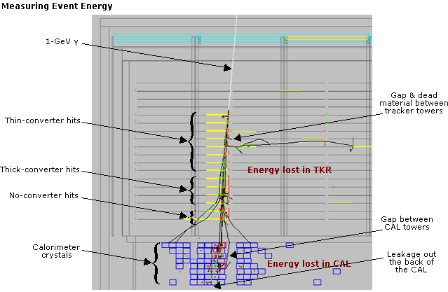
Measuring Energy Deposit in the CAL
Three methods are used to measure the energy deposit in the calorimeter:
- Parametric Correction (can be used for any track).
- Use the tracks to characterize the shower by:
- Position, angle
- Radiation lengths traversed
- Proximity to gaps
- Correct "raw" energy.
- Use the tracks to characterize the shower by:
- "Likelihood" (limited energy and angular range).
- Uses the relation between energy deposit in the last layer and in the rest of the shower.
- Profile Fitting (limited angular range).
- Fit layer-by-layer deposit to shower shape.
Note: Below ~50 GeV, last-layer energy is proportional to the leaked energy.
Note: Best if shower peak is contained in the calorimeter.
Choose the best answer (based on the expected error for each of the three methods).
See Doxygen (latest): AcdRecon
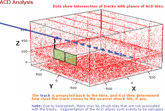
ACD Analysis
The ACD is approximately 99.97% efficient for minimum-ionizing particles (MIPs). However, there are places where, because of gaps in the ACD coverage, charged tracks may fail to produce a signal in any tile. The ACD analysis identifies these gaps to remove sources fo background.
Data Processing Steps (from Inst. Data Analysis Primer):
Raw data sets (LDF.FITS) are translated into FITS format, which is readable by the reconstruction digi.root reconstruction software. Digi.root data is then processed with calibration software to generate the calibration constants files. The constants files are loaded into the primary SAS database (???) , which provides a format-independent interface to allow the reconstruction software to retrieve constants when needed. The reconstruction software produces calibrated data files (recon.root).
==========================================================
Alignment Constants File:
Elements subject to alignment:
| Tower | |
| Trays | Can be displaced with respect to the tower |
| Face | (bottom or top) Can be displaced with respect to the tray. |
| Ladders | Can be displaced with respect to the face. |
| Wafers | Can be displaced with respect to the ladder. |
Example (for simulation):
Tower 3 Tray 1 Face 1 Face 2 Tower 4 Face 0 Ladder 1 Wafer 2 Wafer 1 Notes:
- If no constants are given, zeros are assumed.
- At each level:
- Alignment constants at that level, if any, are read in.
- Constants are merged with those from the level above
(including nulls for any not specified).- The merged constants are passed down to the next level; an array containing one entry for each wafer in the detector – 9216 in all for the flight instrument. Treatment is general; two towers is a special case.
??????????
- Edge Hits
- Interactions in silicon
- Nearly horizontal tracks ???????????
???How it's done:
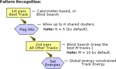
- Perform standard pattern recognition
- Pick tracks (minimum number of clusters in reference and target tower)
- Separate tracks into two parts
- Reference tower (Refit, using only the clusters in that tower)
- Target tower:
- Store measured position and covariance matrix for each hit plane.
- Replace fit position with extrapolation of reference track.
- Accumulate events
- Perform minimization (Minuit)
- Vary parameters in n-dimensional space (n<=6)
- For each set of parameters, transform measwued positions using existing tools.
- Calculate residuals and chi-squared, using weights deerived from covariance matrix and measured errors.
- Compare results with inputs. (Note to self: for test purposes only???)
==========================================================
Ground-based Software
Reconstruction/Simulation Toolkit |
||
Package |
Description |
Provider |
ACD, CAL, TKR RECON |
Data Reconstruction |
LAT |
ACD, CAL, TKR Sim |
Instrument Simulation |
LAT |
GEANT4 |
Particle Transport Simulation |
G4 Worldwide Collaboration |
XML |
Parameters |
World Standard |
ROOT 4.02.00 |
C++ Object I/O |
HEP Standard |
Gaudi |
Code Skeleton |
CERN Standard |
Doxygen |
Code Documentation Tool |
World Standard |
Visual C++/gnu |
Development Environments |
World Standards |
CMT |
Code Management Tool |
HEP Standard |
ViewCVS |
CVS Web Viewer |
World Standard |
CVS |
File Version Management |
World Standard |

|
Between collection and delivery, raw data is transferred from the mission operations center (MOC) to the ISOC where it is unpacked and processed through the pipeline, before being transferred to the GLAST Science Support Center (GSSC) for widespread distribution. To ensure quality, intermediate products are monitored throughout the entire data processing chain. Raw data received from the satellite's downlink telemetry and converted to Level 0 data is input to the GLEAM reconstruction application. |
Gleam Reconstruction Application
Data Flow in the Gaudi Framework

|
The Gleam application finds charged tracks in the tracker and clusters of energy deposition in the calorimeter. The tracks are extrapolated to the ACD to determine whether a tile fired along the path of the track. Potential photons, consisting of two tracks in a "vee" (or possibly a single track, for some high energy photons), are written to an output file where they are available for further analysis. At this stage, cuts can be made to reject background events. |
An I/O and analysis package called ROOT allows C++ objects to be stored inside a file. The ROOT I/O package is designed to create compact files, as well as allow for efficient access to the data. The tree structure of the ROOT files allows a subset of the branches to be manipulated, reducing the amount of I/O required. A C++ script extracts likely photon events and creates a new truncated ROOT file. (See Fig. 1, "Logical structure of the raw data stored in ROOT".)
ROOT files containing data (whether from the satellite, simulation software, or some other source, e.g., beam test data) all have the same internal structure, allowing I/O and low-level analysis routines to be shared. Detailed Monte Carlo truth, detector digitization, and reconstruction data are stored in ROOT files. (See Fig. 2, "Data flow from simulations and the ??? through reconstruction".)
Note the function of RootWriter (which converts ??? files into ROOT files) in Fig. 2. The various formats are converted into C++ objects that are then stored in a ROOT file within its tree structure, with the same event structure used for both real and simulated data. This allows easy comparison between the two. After processing the digitized data, the reconstruction routines produce a Recon ROOT file and a summary file (also in ROOT format, and containing the results of the reconstruction).
Recon
Event reconstruction:
- Takes digitizations from the detector elements.
- Converts them into physics units (e.g., energies in MeV, distances in mm).
- Performs pattern recognition and fitting to find tracks and then photons in the tracker.
- Finds energy clusters in the calorimeter and characterize their energies and directions.
Note: Tracks that extrapolate to a fired ACD tile can be identified.
TKER Tower
A tracker tower consist of strips of silicon detectors arranged in pairs, with each element of the pair providing a separate measurement in one direction (X or Y) perpendicular to the tower axis. Reconstruction is initally done in separate Z-X and Z-Y projections. Projections are associated with each other whenever possible by matching tracks with respect to length and starting positions.
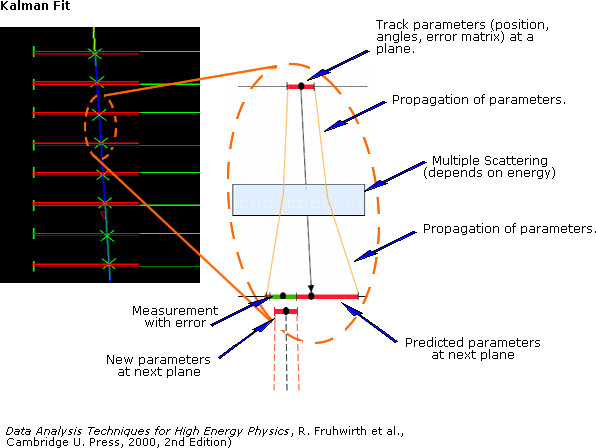
Multiple Coulomb Scattering (MS). In the absence of interactions, particle trajectories would be straight lines. However, the converter foils needed to produce the interactions (as well as the rest of the material in the detector), cause the particle to under go multiple Coulomb scattering (MS) as they traverse the tracker, complicating both pattern recognition (i.e., finding the particles) and track fitting (determining the particle trajectories), particularly for low-energy electrons and positrons. Pattern recognition must therefore be sensitive to particles whose trajectories depart significantly from straight lines.
The presence of multiple scattering also has implications for the fitting procedure. Without MS, deviations from a straight line are due solely to meeasurement errors, which occur independently at each measurement plane and are distributed about the true straight track. In the presence of MS, there are real random deviations from a straight line,and these deviations are correlated from one plane to the next. For example, if an individual particle scatters to the right at one plane, it is more likely to end up to the right of the original undeviated path than to the left.
Covariance Matrix. These correlations can be quantified in a covariance matrix of the measurements, which is caluclated from the momentum of the particle and thte amount of scattering materal between the layers. The dimension of this matrix is the number of measurements. Solving for the track parameters in terms of the mesurements involves inverting this matrix. If ther is no MS, the matrix is diagonal, and the inversion is trivial; MS introduces off-diagonal elements, which complicates the inversion.
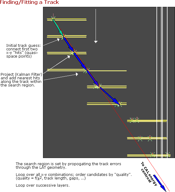
Kalman Filter (KF). The Kalman Filter technique can be useful in both stages of particle reconstruction. First, the initial position, direction, and energy of the particle is estimated. The energy of the particle is based on the response of the calorimeter, and the starting point and direction are derived by looking for three successive hits that line up within some limits.
From this starting point, the track is extrapolated in a straight line to the next layer. Using the estimate of the energy and the amount of material traversed, a decision is made whether the hit in the next layer is within a distance from the extrapolated track allowed by the expected multiple scattering and the uncertainty of the initial estimate. If so, the hit is added to the track, and the position and direction of the track at this plane are modified, incorporating the information from the newly added hit.
The modified track is now extrapolated to the next plane, and the process continues until there are no more planes with hits. All the correlations between layers have been properly taken into account but, at each step, only MS between two successive planes need be considered, and the covariance matrix required is that of the parameters.
The track parameters at the last hit have now been calculated using the information from all the preceding hits. To get the best estimate of the initial direction of the photon, however, it is necessary to know the parameters at the first hit, close to the point where the photon converts to an electron-positron pair.
Smoothing. At this point, smoothing is applied, i.e., the KF is "run backwards" from the last plane to the first, using the appropriate matrices. After smoothing, the track parameters, and their errors have been calculated at each of the measurement planes; in particular, the first plane.
Fig. 3 shows the result of the fitting algorithm applied to a cosmic ray track. "Fit to a cosmic ray track (solid line) in the tracker. Reconstructed energy centroids in the calorimeter (boxes) line up with the track. The track extrapolates to the fired ACD tile."
Calorimeter
A high-energy photon traversing material loses its energy by an initial pair-production process
(λ → e+e-) followed by subsequent bremsstrahlung (e → λ) and pair production, resulting in an electromagnetic cascade, or shower. The scale length for this shower is the radiation length, the mean distance over which a high-energy electron loses all but 1/e of its initial energy.
The calorimeterprovides information about the total energy of the shower, as well as the position and direction , and shape of the shower; or of the penetrating nucleus or muon. It consiststs of eight layers of ten CsI(TI) crystals ("logs") in a hodoscopic arrangement, e.e., alternatively oriented in X and Y directions, to provide an image of the electromagnetic shower. It is designed to measure photon energies from 20 MeV to 300 GeV and beyond.
To comfortably contain photons with energies in the 100-GeV range requires a calorimeter at least twenty radiation lengths thick. However, weight constraints forced limiting Fermi's calorimeter to only ten radiation lengths in thickness; thus, it cannot provide good shower containment for high-energy photons, even though they are very precious for several astrophysics topics.
The mean fraction of the shower contained at 300 GeV is about 30% for photons at normal incidence, at which the energy observed is very different from the incident energy; the shower development fluctuations become larger, and the resolution quickly decreases.
Correcting for Shower Leakage: Method 1 (Shower-profiling). Fit a mean shower profile to observed longitudinal profile. The profile-fitting method proves to be an efficient way to correct for shower leakage, especially at low-incidence angles when the shower maximum is not contained. After the correction is applied, the resolution (as determined from a simulation) is 18% for on-axis TeV photons – animprovement by a factor of two over the result of correcting the energy with a response function based on path length and energy alone.
Correcting for Shower Leakage: Method 2 (Leakage-correction). Use the correlation between the escaping energy and the energy deposited in the last layer of the calorimeter. The last layer carries the most important information concerning the leaking energy: the total number of particles escaping through the back should be nearly proportional to the energy deposited in the last layer.
Both correction methods significantly improve the resolution. The correlation method is more robust, since it does not rely on fitting individual showers, but its validity is limited to relatively well-contained showers, making it difficult to use at more than 70 GeV for low-incidence-angle events. There is still some room for improvement in energy reconstruction especially by correcting for losses in the passive material between the different calorimeter modules and out the sides.
Event Selection
Background rejection performs the function of particle identification, determining whether the incoming particle was a photon.With the hich charged-particle flux in space, shower fluctuations in background interactions can mimic photon showers in non-negligible numbers. Cuts are a pplied to the events to suppress the background.
Description of an implementation of a set of simple and intuitive cuts basted partly on previous experience with EGRET: First, all events are reconstructed, but only events in which none of the ACD tiles fired are considered. (Note: This cut could be applied before any reconstruction, but reconstructing all events is useful in comparing the data with simulations.) The cut eliminates 90% of triggered events. Most of the rejected events consist of charged particles, but a few legitimate photons are also rejected if, for example, one of the particles in the shower exits the detector through the sides or top, and fires an ACD tile.
Next, the reconstructed tracks are tested for track quality, formed from a combination of goodness-of-fit, length of track, and number of gaps on the track. Also, an energy-dependent cut removes events with tracks that undergo an excessive amount of scattering.
Finally, it is required that there be a downward-going vee in both views, and that both tracks in the vee extrapolate to the calorimeter. (This will introduce some inefficiency for high-energy photons, and for highly asymmetric electron-positron pairs. Vees with opening angles that are too large, >60o, are rejected. Such vees generally come from photons with energies below the range of interest.)
=====
Other development paths: additional cuts involving extra particles in the event and extra hits not associated with tracks. ======= looking at the spatial distribution of energy in the calorimeter as a way of distinguishing electromagnetic from hadronic showers, and from the showers of photons traveling upward through the instrument.
Fig. 4 shows a photon that converts in the tracker and deposits energy in the calorimeter. "a reconstructed photon. Note the vee in the tracker, the energy deposited in the calorimeter, and the absence of any signals in the ACD.
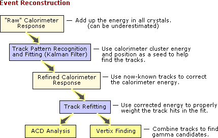
Event Reconstruction in a Nutshell - Toby (Baseline-Preliminary Design Review, Jan 9, 2002)
- Sequence of operations, each implemented by one or more Algorithms, using TDS for communication.
- Trigger analysis: is there a valid trigger?
- Preliminary CAL to find seed for tracker.
- Tracker recon: pattern recognition and fitting to find tracks and then photons in the tracker (uses Kalman filter).
- Full CAL recon: finds clusters to estimate energies and directions.
- Must deal with significant energy leakage since only 8.5 X0 thick.
- ACD recon: associate tracks with hit tiles to allow rejection of events in which a tile fired in the vicinity of a track extrapolation.
- Background rejection: consistency of patterns:
- Hits in tracker.
- Shower in CAL: alignment with track, consistency with EM shower.
| Owned by: |