Lossless Data compression



What is lossless data compression ?

In general, the method of data compression could be divided into two groups, lossless and lossy compression. the method of lossless compression allows to reduce the data size without losing any information. This method is used in making ZIP and GIF files. These differs from the files offered by the method of lossy compression,which loses some information as the JPEG files.



Why we use lossless data compression ?

Whenever we have the problem of space but we don't want to loss any information, we can use losseless compression method. In case of CMS experiment, we propose to take lossless compression in time domain because it allows to reconstruct the original frame. This reconstruction allows to process the time frame with sophisticated offline methods (jitter correction, pile-up study)



Algorithms for the lossless compression and Estimation of the compression factors

we introduce five types of data compression algorithms which are most commonly used in the communication systems or in archiving the data files of the computers. We apply these methods to the ECAL data and evaluate the corresponding compression factors.
There is list of lossless compression methods we have studieds.

Family	Variations
Differential coding	DPCM (Differential Pulse Code Modulation) PDPCM (Predictive Differential Pulse Code Modulation)
Entropy coding	Huffman coding with fixed table Huffman coding with variable table
Transformation coding	Wevelet coding DCT(Discrete Cosine Tansformation) coding
Dynamic coding	None
Residual parametric coding	None
Run-Length coding	Mixed coding with Run-Length and 8 bits coding
Dictionary method	ALDC(Adaptive Lossless Data Compression) DCLZ(Data Compression Lempel-Ziv)

Differential coding

The signal from a given crystal is shaped by the preamplifier so that a decaying time of about 300 ns is introduced. A sampling is performed every 25 ns and the measured voltage is digitized by a 12-bit ADC after passing through the floating point unit(FPU) which determines the dynamic range of the output signal. Fig.1(a) shows the typical shape of the signal and the points of samplings in unit of 25 ns. The hights of the signal at the sampling points are recorded. Another possible way of keeping the same amount of information is to record the value at the first sampling point and then to record the difference between the first and the second, between the second and the third, and so on. This method is called the differential coding. The advantage of such a coding scheme is that the numbers to record are usually smaller than the standard coding, and the number of bits needed to record the numbers may be smaller even though we need to introduce one more bit that represent the sign of the differences which can be negative. Fig.1(b) shows the differences between two neighboring samples. This simple method allows us to reduce the length of the data, especially if the signal varies slowly with respect to the sampling interval. In our case, however, the rise and fall of the signal is so fast that no signaificant gain in the data length may be expected. Nevertheless, it will be instructive to do an exercise and estimate the compression rate using the data of Fig.1. The number of bits needed to code the sampled value x(i)is given by Int(log2(x(i))+1),whereas the difference between the neighboring samples d(i) = x(i) - x(i+1) can be coded by Int(log2(abs(d(i)+0.5)+1)+1)+1 bits. These numbers of bits corresponding to the 14 sampling values and also to the differences are given in Table 1. The maximum number of bits in the two cases are 12 and 11, respectively, and no significant gain is achieved by applying this algorithm.

Samplings	1	2	3	4	5	6	7	8	9	10	11	12	13	14
Normal coding	7	11	11	11	12	11	11	11	10	10	9	8	8	7
Differencial coding	11	11	9	7	9	10	10	10	10	9	9	8	8	-

Table 1:Number of bits needed to record the differences between the neighboring sample values



Fig.1(a) Differential coding: Shape of the signal vs. time



Fig.1(b) Differences between neighboring samples



Residual parametric coding :

If the shape of the signal has a time dependence that can be approximated by a simple function of time, and if the difference between the signal and the function is small in most of the cases, we may reduce the data size by coding the differences. To apply this algorithm called residual parametric coding, we proceed as follows :

   (1) Generate a model as shown in Fig.2(a)
   (2) Normalize the model to the signal so that the maxima of the
        two have the same magnitudes. See Fig.2(b)
   (3) Calculate the differences between the signal and the model
        at the sampling points.
   (4) Make the data file of the following structure.

Here, the header represents the maximum bit length, Nb, of the difference values. The header is followed by the value of the signal at its maximum, and then by the difference values having Nb bits each. Using the data and the model function shown in Fig1(c) and Fig1(d), we obtain the Table 2. As we have 16 samples of 12 bits, the initial length is 192 bits. With this residual parametric coding, only 106(4+12+15*6) bits are needed, giving a compression factor of 1.79.

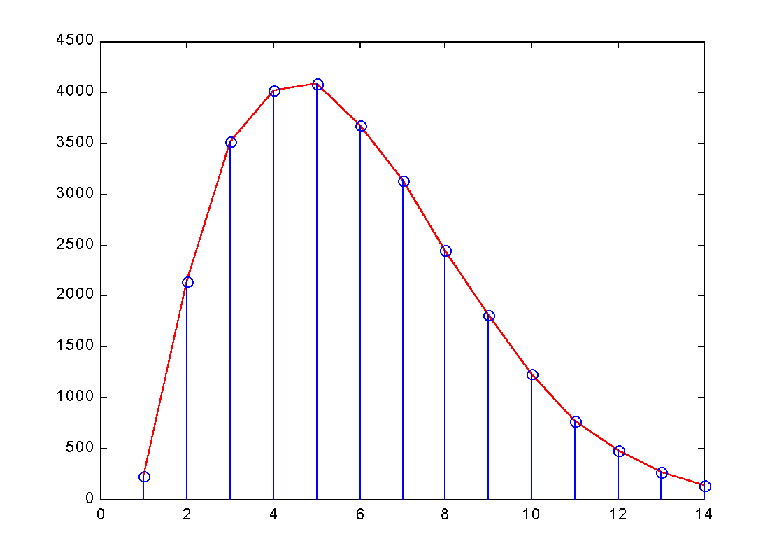
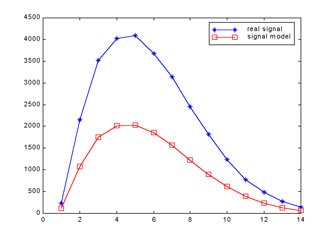
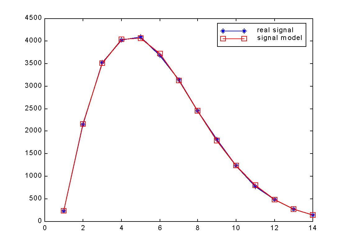
Samplings	1	2	3	4	5	6	7	8	9	10	11	12	13	14	15
Normal coding	12	12	12	12	12	12	12	12	12	12	12	12	12	12	12
R.P.C.	2	4	4	5	6	5	3	5	1	6	3	3	5	5	5

Table 2: Number of bits needed to record the differences between the signal and the model




Fig.2(a) Residual parametric coding: Signal and Model before normalization



Fig.2(b):Signal and Model after normalization



Huffman coding :

When the same numbers appear repeatedly, we may replace these numbers with some other numbers having shorter number of bits. The best reduction of the total length of a set of numbers can be obtained by associating more frequently apprearing numbers to shorter numbers. Huffman's coding method gives the optimized assignment rule which is uniquely decodable[9]. We take an example of Huffman coding to illustrate this method. Let us consider a set of 6 numbers A_i, ( i =1,.. 6) occurring with the probabilities 0.4, 0.3, 0.1, 0.1, 0.06, 0.04, respectively. The corresponding Huffman codes are given in Table3.

Number	Probability	Code
A1	0.4	1
A2	0.3	00
A3	0.1	011
A4	0.1	0100
A5	0.06	01010
A6	0.04	01011

Table 3:An example of Huffman code assignment


The average length of this code is 0.4 X 1 + 0.3 X 2 + 0.1 X 3 + 0.1 X 4 + 0.06 X 5 + 0.04 X 5 = 2.2 bits/number whereis the fixed length coding requires at least 3 bits for each number. Once the code is fixed, the coding and decoding are done in a unique way. The numbers are written in a form of a block code. For example, the sting 01000101001100 is unambiguously decoded as A₄ A₅ A₃ A₂.
To apply the Huffman coding method to the ECAL data, we used the distribution of the ADC counts shown in Fig.3(a). The shortest Huffman code is associated to the most frequently occurring value IP. To the ADC values from IP-7 to IP+7 are assigned the codes with its length varying from 2 to 9 bits. For the values smaller than IP-7, a 9+8 bits structure is used, where the Huffman code of 9 bits is followed by the 8 lowest bits of the ADC. For the values larger than IP+7, a 4+16 bits structure is used, making use of the full 16 bits of the ADC. The resulting Huffman code assignment is given in Table 4.

ADC Counts	Probability	Code	Word length
IP-8 or smaller	0.19	0000	4+16
IP-7	0.22	101101001	9
IP-6	0.42	10110101	8
IP-5	0.78	1010101	7
IP-4	1.72	101100	6
IP-3	4.42	10111	5
IP-2	10.10	001	3
IP-1	17.40	110	3
IP	21.05	01	2
IP+1	17.69	111	3
IP+2	10.74	100	3
IP+3	5.19	0001	4
IP+4	2.53	10100	5
IP+5	1.46	101011	6
IP+6	0.95	1011011	7
IP+7	0.67	1010100	7
IP+8  or larger	4.46	0000	4+16

Table 4: Huffman code assignment for the ECAL ADC values, Here IP respresents the ADC value corresponding to the pedestal, which is 25 in this case

Table 5 shows the performance of the Huffman coding for the 100 hard QCD events with five different SR types. A good performance of compression is obtained with this truncated Huffman method. Also shown in the same table is the compression factors obtained by applying the unix command $compact$ that uses an adaptive Huffman code.

SR type	event size	Huffman coding	compact
SR1(time+space)	41.2 kB	10.4 kB(4.1)	13.7 kB(3.0)
SR2-1(time, Et>2.5 GeV)	29.8 kB	7.6 kB(3.9)	9.5 kB(3.1)
SR2-2(time, Et>1.0 GeV)	138.9 kB	33.0 kB(4.2)	49.0kB(2.83)
SR2-3(time, Et>0.5 GeV)	381.4 kB	87.0 kB(4.3)	129.2.0kB(2.9)
SR2-4(time, Et>0.3 GeV)	662.8 kB	148.0 kB(4.4)	221.0 kB(2.9)

Table 5: The event sizes with and without Huffman coding. Results with the Truncated Huffman coding using a fixed table and the Adaptive Huffman coding with a variable table are shown.


Fig 3.(a)Distribution of the ADC counts used to generate the Huffman codes (b) Same distribution with barrel (c)Same distribution with endcaps


Dictionary method:

The dictionary method uses the property of many data types that contain repeating code sequences. It can be divided into two main groups which are based on the algorithm developed and published by A. Lempel and J. Ziv[10]. The point of the first group is to try to find if the character sequence currently being compressed has already occurred earlier in the input data. In the case the same sequence is found, instead of repeating it, the algorithm outputs a pointer. See Fig.4(a).The second group creates a dictionary of the phrases that occur in the input data. When they encounter a phrase already present in the dictionary, they just output the index number of the phrase in the dictionary as shown in Fig.4(b)[14]. In most of the unix machines, the commands compress and gzip performs the compression using the dictionary method. Therefore, we have evaluated the compression rates using the simulated ECAL data in the two cases. The results that we obtain for different SR criteria are summarized in Table 6.

SR type	event size	compress	gzip
SR1(time+space)	41.2 kB	11.6 kB(3.5)	12.0 kB(3.4)
SR2-1(time, Et>2.5 GeV)	29.8 kB	8.0 kB(3.7)	8.3 kB(3.6)
SR2-2(time, Et>1.0 GeV)	138.9 kB	38.9 kB(3.5)	41.50kB(3.3)
SR2-3(time, Et>0.5 GeV)	381.4 kB	99.7 kB(3.8)	106.8.0kB(3.6)
SR2-4(time, Et>0.3 GeV)	662.8 kB	168.6 kB(3.9)	184.0 kB(3.6)

Table 6: The compression factors for the ECAL data using the unix commands



Fig 4.Dictionary methods: (a)scheme 1 and (b)scheme 2


Dynamic coding :

It was suggested by Busson et al[11] that a reduction of the data size can be done by simply choosing the word length between one byte and two bytes. In this dynamic coding scheme, the first one or two bits of the 8 bits is used to indicate the length of the signal from each crystal. A slightly modified data structure is described in the following.
The energies of the 25 crystals in a given trigger tower are stored in consecutive. The 10 values corresponding the ten time samplings for the first crystal are written first, followed by the 10 time samplings of the next crystal, etc. By allocating one byte(eight bits) to each energy value, a minimum of 250 bytes are needed to record all the energy values. If a crystal has an energy exceeding the maximum that can be represented by the eight bit, one more byte or two is used. The number of crystals that need two or three bytes and their sequential number are also coded in the data train. These numbers can be represented by a one byte. We suggest the data structure as described below.

(1) In the first byte, the first bit(MSB) is used to specify the data type: either full ten time samplings or the filtered value. The next bit is reserved as the flag of the presence of very large signal which needs 3 bytes. The remaining 6 bits are used to assign the position in Eta of the corresponding trigger tower which varies from 1 to 56.
(2) The first bit of the next byte indicates the presence of the 2- byte data, and the following seven bits specify the position in phi ranging from 1 to 72.
(3) In the case that 2-byte data are present, the number of the crystals which recorded such signals is written in the next byte. Let's call it N₂ (N₂ =0,..250). This byte can be followed by another byte, which is, N₃, if necessary.
(4) The sequential numbers of the crystals that need 2-byte record occupy N₂ bytes. Sometimes it can be followed by N₃ addresses for crystals having very high energy deposit.
(5) Total of 250 + N₂ + N₃ * 2 bytes to record the ADC counts of a trigger tower chosen by the SR.

In the case that we use the space domain data to get a better reduction rate, we read the sum over ten samplings if the transverse energies of a tower is between 1.0 GeV and 2.5 GeV. The event sizes with and without dynamic coding are given in TableY1 for various SR parameters. About a factor of two compression is obtained, as expected.

SR type	event size	dynamic coding	compression factor
SR1(time+space)	41.2 kB	21.0 kB	1.9
SR2-1(time, Et>2.5 GeV)	29.8 kB	15.0 kB	1.9
SR2-2(time, Et>1.0 GeV)	138.9 kB	69.8 kB	1.9
SR2-3(time, Et>0.5 GeV)	381.4 kB	191.7	1.9
SR2-4(time, Et>0.3 GeV)	662.8 kB	333.0	1.9

Table 7:The event sizes with and without dynamic coding.

---

Back ECAL Home